Predicting Ionic Liquid Melting Points: A Comprehensive Guide to QSPR and Machine Learning Models
Accurate prediction of ionic liquid melting points is critical for tailoring their properties in applications ranging from energy storage to pharmaceutical development.
Predicting Ionic Liquid Melting Points: A Comprehensive Guide to QSPR and Machine Learning Models
Abstract
Accurate prediction of ionic liquid melting points is critical for tailoring their properties in applications ranging from energy storage to pharmaceutical development. This article provides a comprehensive overview of Quantitative Structure-Property Relationship (QSPR) models and machine learning approaches for melting point prediction. It covers fundamental principles, state-of-the-art methodologies, optimization strategies to overcome data sparsity and model reliability challenges, and rigorous validation techniques. Designed for researchers, scientists, and drug development professionals, this resource synthesizes current research trends and practical guidance to facilitate the efficient design and selection of ionic liquids with desired phase behavior, reducing reliance on costly experimental screening.
The Fundamentals of Ionic Liquids and Why Melting Point Prediction Matters
FAQs: Ionic Liquids and Melting Point Characterization
Q1: What defines an ionic liquid and why is its melting point a critical property? An Ionic Liquid (IL) is broadly defined as a salt in which the ions are poorly coordinated, leading to a melting point generally below 100 °C. Many are liquid at room temperature. Their low melting point is a direct consequence of the bulky and asymmetric structure of the constituent organic cations, which prevents the ions from packing efficiently into a crystal lattice [1] [2] [3]. The melting point is a critical property because it defines the lower limit of the liquidus range for applications such as electrolytes in batteries, solvents for chemical reactions, and as functional materials in thermal energy storage [4] [5]. Accurately predicting it is essential for the computer-aided design of new ILs with desired phase behavior [6].
Q2: What are the common experimental challenges when determining the melting point of ionic liquids? Researchers often face several challenges:
- Supercooling: Many ILs tend to supercool, meaning they remain in a liquid state well below their thermodynamic melting point, which can lead to inaccurate measurements [4].
- Polymorphism and Complex Solid-Solid Transitions: Some ILs, especially a subclass known as Organic Ionic Plastic Crystals (OIPCs), can exhibit multiple solid phases with transitions between them before melting. These solid-solid transitions also involve enthalpy changes and must be carefully characterized to avoid confusing them with the final melting point [1] [4].
- Purity and Hygroscopicity: The presence of impurities or absorbed water can significantly alter the measured melting point. Many ILs are hygroscopic and must be handled under strict anhydrous conditions to obtain reliable data [2].
Q3: How can QSPR models assist in the design of ionic liquids with specific melting points? Quantitative Structure-Property Relationship (QSPR) models are computational tools that relate the molecular structure of ILs to their melting points. By using machine learning on datasets of known ILs, these models identify which molecular descriptors (e.g., ion size, symmetry, types of chemical bonds) most significantly influence the melting point [6] [5]. This allows researchers to predict the melting points of vast numbers of theoretical cation-anion combinations (e.g., over 35,000) before undertaking costly synthesis, thereby speeding up the discovery of ILs with tailored properties [6].
Q4: What are some key molecular features that generally lead to a lower melting point in ILs? Several structural features are known to depress the melting point of ILs:
- Large Ion Size and Asymmetry: Bulky, asymmetrical cations (like imidazolium with long alkyl chains) prevent efficient crystal packing [1] [3].
- Charge Delocalization: Anions where the negative charge is spread over a larger area (e.g., bis(trifluoromethylsulfonyl)imide, [NTf₂]⁻) weaken the Coulombic forces between ions [4].
- Flexible Alkyl Chains: Chains on the cation can introduce conformational disorder, inhibiting crystallization [4].
- Weak Hydrogen Bonding Ability: Reducing the strength of hydrogen-bonding networks between the cation and anion can lower the melting point [4].
Troubleshooting Guide: Melting Point Experiments
| Common Problem | Potential Cause | Recommended Solution |
|---|---|---|
| High Supercooling | High viscosity, slow nucleation kinetics, impurity effects. | Seed the sample with a tiny crystal of the solid phase. Use a slower cooling rate prior to measurement [4]. |
| Broad or Ill-Defined Melting Endotherm | Sample impurity, decomposition upon heating, polymorphism, or non-equilibrium conditions. | Purify the IL (e.g., recrystallization, washing). Ensure anhydrous handling. Use multiple heating/cooling cycles to establish reproducibility [2] [4]. |
| Discrepancy between Calculated and Experimental Tm | Inaccuracies in the QSPR model, insufficient training data for the specific IL family, or unaccounted for ion-pairing in the liquid state. | Verify the IL's chemical structure and purity. Use a QSPR model that has been validated for the specific cation/anion classes of your IL. Consult the model's applicability domain to ensure your IL is within its reliable prediction space [6] [5]. |
| Corrosion of Metal Sample Containers | Chemical reactivity of the IL anions (e.g., halides) with metal surfaces at elevated temperatures. | Use containers made of inert materials such as Teflon, quartz, or certain types of stainless steel with proven compatibility [4]. |
Essential Data for Ionic Liquid Melting Points
Table 1: Melting Points and Enthalpies of Common Imidazolium-Based Ionic Liquids [4]
| Ionic Liquid | Cation Abbr. | Anion Abbr. | Melting Point Range (°C) | Enthalpy of Fusion (kJ/kg) |
|---|---|---|---|---|
| 1-Hexadecyl-3-methylimidazolium Bromide | [C₁₆MIM] | Br | ~64 | 159.00 |
| 1-Hexadecyl-3-methylimidazolium Chloride | [C₁₆C₁IM] | Cl | ~64 | 159.00 |
| Various Imidazolium ILs | [CₓMIM] | [NTf₂], [TfO], etc. | -87 to 208 | 59.00 - 159.00 |
Table 2: Performance Metrics of a Deep-Learning Model for Melting Point Prediction [5]
| Model Type | Dataset Size | R² Score | Root Mean Square Error (RMSE) |
|---|---|---|---|
| Deep Learning (RNN) | 1253 ILs | 0.90 | ~32 K (~32 °C) |
Experimental Protocol: Determining Melting Point via DSC
Objective: To accurately determine the melting point (Tm) and enthalpy of fusion (ΔHf) of an ionic liquid using Differential Scanning Calorimetry (DSC).
Materials and Equipment:
- Differential Scanning Calorimeter
- Hermetically sealed, inert sample pans (e.g., aluminum Tzero)
- Micro-syringe or spatula for sample handling
- Glove box (for hygroscopic or air-sensitive ILs)
- Pure, dry ionic liquid sample
Procedure:
- Sample Preparation: Inside a glove box if necessary, accurately weigh 5-10 mg of the pure, dry IL into a pre-tared DSC sample pan. Seal the pan hermetically to prevent moisture ingress or solvent evaporation during the experiment.
- Instrument Calibration: Calibrate the DSC cell for temperature and enthalpy using high-purity standards such as indium or zinc.
- Experimental Method:
- Loading: Place the sealed sample pan and an empty reference pan in the DSC cell.
- Thermal Program:
- Equilibrate at 25 °C.
- Cool to -100 °C at a rate of 10 °C/min.
- Hold isothermally for 5 minutes to ensure thermal equilibrium.
- Heat to 150 °C at a scan rate of 5 °C/min. This slower heating rate is recommended to minimize thermal lag and better resolve complex thermal events like solid-solid transitions.
- Repeat: Perform at least two full heating/cooling cycles to establish the reproducibility of the thermal events.
- Data Analysis:
- On the final heating scan, identify the onset temperature of the endothermic peak corresponding to melting; this is reported as the melting point (Tm).
- Integrate the area under the melting peak to determine the enthalpy of fusion (ΔHf).
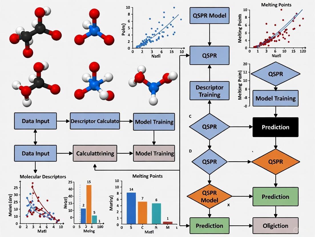
QSPR Workflow for Melting Point Prediction
The following diagram illustrates the workflow for developing a QSPR model to predict the melting points of Ionic Liquids.
Table 3: Essential Materials for IL Synthesis and Melting Point Analysis
| Item Name | Function/Description | Example in Context |
|---|---|---|
| Imidazolium Cations | A common class of organic cations providing a versatile, tunable platform for IL synthesis. | 1-Butyl-3-methylimidazolium ([C₄MIM]⁺) is a widely studied cation whose salts often have low melting points [4]. |
| Complex Anions | Inorganic or organic anions that contribute to charge delocalization and low lattice energy. | Bis(trifluoromethylsulfonyl)imide ([NTf₂]⁻) and tetrafluoroborate ([BF₄]⁻) are common anions that help achieve low melting points [4] [5]. |
| Differential Scanning Calorimeter (DSC) | The primary instrument for the experimental determination of melting points and enthalpies of fusion. | Used to measure the precise melting temperature and latent heat of an unknown IL sample for model validation [4]. |
| ILThermo Database | A comprehensive NIST database for collecting experimental thermophysical property data on ILs. | Serves as a critical source of high-quality experimental data for training and validating QSPR models [5]. |
| COSMO-RS Computational Method | A thermodynamic method for predicting chemical potentials and activity coefficients, applicable to ILs. | Can be used to calculate activity coefficients at infinite dilution, which are related to solubility and can inform property models [7]. |
The Critical Role of Melting Points in Application Performance
FAQs and Troubleshooting Guides
This guide addresses common challenges researchers face when determining the melting points of Ionic Liquids (ILs) and how these impact application performance within the context of Quantitative Structure-Property Relationship (QSPR) modeling.
Q: What is the most common error in melting point determination, and how does it affect the result?
A: The most prevalent error is heating the sample too quickly [8]. This causes a thermal lag between the sample's actual temperature and the temperature registered by the thermometer. The consequence is an artificially high and broad melting point range [8]. This inaccurate data can mislead the assessment of an IL's purity and identity, and if used in QSPR model training, can reduce the model's predictive accuracy.
Q: My melting point measurement is broad and inconsistent. What could be the cause?
A: A broad melting range often stems from technique rather than the sample itself. Key factors to check are [8]:
- Heating Rate: Ensure you slow the heating rate to 1-2 °C per minute as you approach the anticipated melting point [8].
- Sample Preparation: The sample must be finely powdered and densely packed into the capillary tube to a height of no more than 2-3 mm [8]. A large or loosely packed sample creates temperature gradients, leading to a broad range.
- Instrument Calibration: An uncalibrated thermometer can introduce a systematic error. Regularly calibrate your apparatus using known melting point standards [9].
Q: How can I determine if a depressed melting point is due to impurity or just poor technique?
A: First, repeat the measurement with careful attention to slow heating and proper sample packing. If the melting range remains broad and depressed, it is a strong indicator of sample impurity. Technique-related errors typically resolve upon careful repetition, while impurity is an intrinsic property of the sample [8] [9].
Q: Why is accurate melting point data critical for QSPR models of Ionic Liquids?
A: QSPR models learn the relationship between molecular descriptors of ions and their measured properties. The presence of erroneous data (e.g., artificially high melting points from rapid heating) introduces "noise" that confuses the model. High-quality, accurate experimental data is the foundation for building robust and reliable QSPR models that can genuinely predict the melting points of new, unsynthesized ILs [6] [5].
Melting Point Errors and Their Impact
The following table summarizes common experimental errors and their consequences for your data and subsequent QSPR modeling.
| Error Type | Consequence on Melting Point | Impact on QSPR Model Development |
|---|---|---|
| Rapid Heating [8] | Artificially high & broad melting range. | Introduces noise, reducing prediction accuracy and model reliability. |
| Improper Sample Packing (too much, not dense) [8] | Broad, uneven melting range. | Obscures the true sharp melting point of pure compounds, affecting data quality. |
| Uncalibrated Thermometer [9] | Systematic high or low readings. | Creates a consistent bias in the dataset, leading to systematically incorrect predictions. |
| Wet or Impure Sample [8] [9] | Depressed (lowered) & broad melting range. | Provides incorrect target values for the model to learn from, confusing structure-property relationships. |
Experimental Protocol: Accurate Melting Point Determination
This protocol ensures the generation of high-quality data suitable for QSPR studies [8] [9].
1. Sample Preparation
- Grinding: Use a clean mortar and pestle to grind the sample into a fine powder.
- Packing: Fill a melting point capillary tube by tapping the open end into the powder. Tap the closed end down on a hard surface or slide the tube down a long glass tube to densify the sample. Repeat until the sample is a compact column of 2-3 mm in height [8].
2. Apparatus Setup
- Place the capillary tube in the melting point apparatus.
- If the approximate melting point is known, heat rapidly to about 15-20 °C below the expected range [8].
3. Measurement and Data Recording
- Once near the melting point, sharply reduce the heating rate to 1-2 °C per minute [8].
- Carefully observe the sample. Record two temperatures:
- Initial Melting Point (T₁): The temperature at which the first drop of liquid is observed.
- Final Melting Point (T₂): The temperature at which the last solid crystal disappears into the liquid [9].
- The melting point is reported as a range: T₁ - T₂.
4. Thermometer Calibration
- Perform regularly using at least two certified melting point standards that bracket your range of interest.
- Measure the melting point of the standards using the protocol above.
- Plot the observed values versus the literature values to create a calibration curve for your specific thermometer [9].
The Scientist's Toolkit: Essential Research Reagents and Materials
| Item | Function in Melting Point Analysis |
|---|---|
| Melting Point Apparatus | A specialized instrument with a heated block, viewer, and temperature control for precise measurement. |
| Capillary Tubes | Thin-walled glass tubes for holding a small amount of the solid sample. |
| Melting Point Standards | Ultra-pure compounds with known, sharp melting points (e.g., vanillin, acetanilide) used for thermometer calibration [9]. |
| Molecular Descriptor Software | Software (e.g., Dragon) used to calculate numerical representations (descriptors) of the cation and anion structure from their SMILES strings for QSPR modeling [5]. |
Workflow for Integrating Experimental Data with QSPR Modeling
The diagram below illustrates the workflow from experimental measurement to QSPR model development and application.
Frequently Asked Questions (FAQs)
1. What is QSPR and how is it used for ionic liquids? Quantitative Structure-Property Relationship (QSPR) is a computational modeling approach that uses mathematical equations to predict the properties of chemical compounds based on their molecular structures. For ionic liquids (ILs), QSPR models establish relationships between molecular descriptors (numerical representations of structural features) and specific IL properties, such as melting point. This allows researchers to predict properties for new, unsynthesized IL combinations, significantly accelerating the design of ILs with tailored characteristics for specific applications like energy storage or catalysis [6] [10].
2. Why is predicting the melting point of ionic liquids important? The melting point (Tm) of an ionic liquid is a critical property that determines its operational temperature range in applications such as batteries, supercapacitors, and industrial extraction processes. A low melting point is often desirable for practical use. However, the Tm can vary dramatically based on the molecular structures of the cation and anion and their combination. QSPR models provide a way to systematically understand and predict Tm, enabling the computer-aided design of ILs with favorable melting points without relying solely on costly and time-consuming experimental synthesis and testing [5].
3. What are the common computational methods used in QSPR for IL melting points? Researchers employ a variety of machine learning and statistical methods to build predictive QSPR models for IL melting points. Commonly used algorithms include:
- Partial Least Squares Regression and Stepwise Multiple Linear Regression for linear modeling [6].
- Monte Carlo optimization using software like CORAL to generate models based on hybrid optimal descriptors derived from molecular structures [11].
- Deep Learning models, which can process a vast number of molecular features and have demonstrated high predictive accuracy for Tm [5].
- Projection Pursuit Regression (PPR), which can capture nonlinear relationships between descriptors and the melting point [12].
4. What molecular features influence the melting point of ionic liquids? QSPR studies have identified several key structural attributes that affect the melting point of ionic liquids. These include:
- Symmetry: Higher molecular symmetry often leads to higher melting points due to better crystal packing.
- Flexibility: The presence of rotatable bonds can lower the melting point.
- Branched chains: Branching in alkyl chains generally decreases the melting point.
- Aromatic systems: The presence of benzene ring structures in cations influences intermolecular interactions and Tm.
- Intramolecular electronic effects: The electronic distribution within the ions affects the strength of Coulombic interactions [12].
Troubleshooting Guides for QSPR Modeling
Issue 1: Poor Model Performance and Low Predictive Accuracy
Potential Causes and Solutions:
Cause: Inadequate or Non-Representative Molecular Descriptors. The set of molecular descriptors used may not sufficiently capture the structural features governing the melting point.
Cause: Overfitting of the Model. The model may perform well on training data but poorly on new, unseen data.
- Solution: Implement a rigorous validation protocol. This should include internal cross-validation and external validation with a separate test set. Always define the model's applicability domain to understand its limitations. Reducing the descriptor dimensionality by removing low-variance or highly correlated features can also prevent overfitting [6] [5].
Cause: Suboptimal Data Splitting. The way the dataset is divided into training, calibration, and validation sets can impact the perceived performance.
Issue 2: Model is Not Robust or Chemically Interpretable
Potential Causes and Solutions:
Cause: Lack of Mechanistic Interpretation. The model predicts the endpoint but offers no insight into which structural features are responsible.
- Solution: Use modeling approaches that allow for mechanistic interpretation. For instance, in Monte Carlo-based models, analyze the correlation weights (CW) of specific structural attributes. Positive CW indicates a fragment increases the property (e.g., melting point), while negative CW indicates a fragment decreases it [10] [11].
Cause: Ignoring the Effect of Chemical Family. The model may not account for variations in performance across different classes of cations and anions.
- Solution: Analyze the model's performance stratified by the chemical family of the ions. Highlighting these effects can provide deeper insights and guide the design of future ILs [6].
Issue 3: Challenges in Handling Ionic Liquid Structures
Potential Causes and Solutions:
Cause: Difficulty in Representing the Ionic Pair. Ionic liquids consist of two distinct ions, and creating a single molecular representation for QSPR can be challenging.
- Solution: Employ and compare different combining rules. These are averaging functions used to obtain the descriptors of the entire IL from the descriptors of the individual ions. Testing different rules is crucial for building a robust model [6].
Cause: Limited Experimental Data for Training. The availability of high-quality, experimental melting point data for a diverse set of ILs may be limited.
- Solution: Leverage large, publicly available databases like ILThermo to compile datasets. For deep-learning models, which require large datasets, this is particularly important [5].
Experimental Protocols: Key Workflows in QSPR for IL Melting Points
Protocol 1: Building a QSPR Model Using Machine Learning
This protocol outlines the general workflow for developing a QSPR model to predict the melting points of Ionic Liquids [6] [5].
- Data Collection: Extract experimental melting point data for ionic liquids from databases (e.g., ILThermo) or published literature.
- Structure Representation and Descriptor Calculation:
- Represent the molecular structures of cations and anions using Simplified Molecular Input Line Entry System (SMILES) notations or draw them with molecular editing software.
- Use software (e.g., Dragon) to calculate a wide range of molecular descriptors for each ion.
- Data Preprocessing and Splitting:
- Preprocess the data by removing descriptors with low variance or missing values.
- Split the entire dataset randomly into a training set (≈80%) and a validation set (≈20%).
- Feature Selection:
- Apply feature selection techniques (e.g., using Pearson correlation matrix) to identify a subset of significant molecular descriptors that are highly correlated with the melting point. Remove descriptors with low correlation (<0.20) or high inter-correlation (>0.90) to prevent overfitting.
- Model Training and Validation:
- Train various machine learning algorithms (e.g., Partial Least Squares, Deep Learning) on the training set.
- Validate the trained model's predictive performance on the separate validation set using statistical metrics like R² and RMSE.
The workflow for this protocol is summarized in the diagram below:
Protocol 2: Building a Model with Monte Carlo Optimization (CORAL Software)
This protocol details the methodology for creating a QSPR model using the Monte Carlo algorithm as implemented in the CORAL software [10] [11].
- Data Compilation: Compile a dataset of compounds with known experimental property values (e.g., melting point, expressed as log H50 for sensitivity, or Tm).
- Structure Representation: Draw molecular structures and convert them into SMILES notations.
- Data Splitting: Randomly divide the dataset into four subsets for a robust modeling process:
- Active Training Set (≈33%): Used for the model's initial training.
- Passive Training Set (≈31%): Used for additional training.
- Calibration Set (≈16%): Used to optimize the model's parameters.
- Validation Set (≈20%): Used for the final, unbiased evaluation of the model.
- Descriptor Calculation and Optimization:
- The CORAL software calculates hybrid optimal descriptors (DCW) from the SMILES notations and/or graph representations via Monte Carlo optimization.
- The optimization process aims to find the best correlation weights for molecular attributes to predict the target property.
- Model Building and Validation:
- Build the QSPR model using the target function and optimized descriptors.
- Validate the model using both internal and external validation parameters (e.g., R²Validation, Q²Validation) from the calibration and validation sets.
- Mechanistic Interpretation: Examine the correlation weights of structural attributes to identify fragments that increase or decrease the target property.
The workflow for this protocol is summarized in the diagram below:
Data Presentation: Model Performance Comparison
The following table summarizes the performance of different QSPR modeling approaches as reported in the literature, providing a benchmark for expected outcomes.
Table 1: Performance Metrics of Various QSPR Models for Ionic Liquid Properties
| Modeling Approach | Property Predicted | Data Points | Key Statistical Metrics | Reference / Software |
|---|---|---|---|---|
| Deep Learning Model | Melting Point (Tm) | 1253 ILs | R² ≈ 0.90, RMSE ≈ 32 K | [5] |
| Monte Carlo Optimization | Melting Point (Tm) of Imidazolium ILs | 353 ILs | R²Validation: 0.78-0.85, Q²Validation: 0.77-0.84 | CORAL Software [11] |
| Projection Pursuit Regression (PPR) | Melting Point (Tm) | 288 ILs | R² = 0.81, AARD* = 17.75% | CODESSA Program [12] |
| Monte Carlo Optimization | Impact Sensitivity (log H50) | 404 Nitro Compounds | R²Validation = 0.78, Q²Validation = 0.77 | CORAL Software [10] |
| Multiple Machine Learning Classifiers | State of Matter (at 300 K) | 953 IL Salts | N/A (Classification) | [6] |
AARD: Average of Absolute Relative Deviation
The Scientist's Toolkit: Essential Research Reagents and Software
Table 2: Key Resources for QSPR Modeling of Ionic Liquids
| Tool Name | Type | Primary Function in QSPR |
|---|---|---|
| CORAL Software | Software | Implements the Monte Carlo algorithm to build QSPR models using SMILES-based optimal descriptors. Used for robust model development and validation [10] [11]. |
| Dragon | Software | Calculates a very large number (5000+) of molecular descriptors from molecular structures, which are used as inputs for machine learning models [5]. |
| ILThermo Database | Database | A comprehensive NIST database for experimentally measured thermodynamic properties of ionic liquids, serving as a key source for training data [5]. |
| SMILES Notation | Representation | A string-based representation of molecular structure that serves as input for descriptor calculation in software like CORAL and for converting IUPAC names [10] [5]. |
| OPSIN Library | Software Library | Used to convert IUPAC names of chemical compounds into SMILES representations, facilitating the processing of large datasets [5]. |
Key Molecular Descriptors for Characterizing Cations and Anions
Frequently Asked Questions (FAQs)
FAQ 1: What is the most effective way to represent the structure of an ionic liquid for calculating molecular descriptors? The structure of an ionic liquid can be represented in two primary ways for descriptor calculation: using descriptors derived for separate ions or for the whole ionic pair [13] [14]. A benchmark study concluded that a description based on 2D descriptors calculated for ionic pairs is often sufficient to develop a reliable QSPR model. This approach yields high accuracy in both calibration and validation, and it streamlines the descriptor selection process by reducing the number of potential variables at the start of model development [13] [14]. While many models use 3D descriptors from separately optimized ion geometries, 2D descriptors derived from the structural formula are less time-consuming and can be just as effective without significant loss of model quality [14].
FAQ 2: How does the choice of geometry optimization method affect my QSPR model? The level of theory used for geometry optimization can significantly influence the values of 3D molecular descriptors and, consequently, the quality of the final QSPR model [13] [14]. Research has shown that descriptor values are dependent on the applied theory level [14]. Models utilizing descriptors from molecular geometries optimized with semi-empirical PM7 and ab initio Hartree-Fock (HF/6-311 + G) methods often show similarly high quality and validation parameters [14]. In contrast, models based on geometries from more computationally intensive methods like Density Functional Theory (DFT with B3LYP/6-311 + G) can sometimes result in lower model quality [14]. Therefore, the semi-empirical PM7 method is frequently recommended for the routine optimization of anion and cation geometries [14].
FAQ 3: What are "combining rules" and why are they important in QSPR for ionic liquids? Combining rules are defined as averaging functions used to obtain the molecular descriptors of an entire ionic liquid from the descriptors calculated for its individual ions [6]. The choice of rule is a key novelty in recent QSPR models and is critical for checking model robustness [6]. Since ionic liquids are composed of disconnected cations and anions, a rule is required to aggregate their independent descriptor values into a single set that represents the salt. Investigating different combining rules is part of a good practice protocol in QSPR model selection [6].
FAQ 4: Which machine learning algorithms are commonly used in QSPR models for properties like melting point? A variety of machine learning algorithms are successfully applied in QSPR studies for ionic liquids. These include both regression and classification methods [6]. Common algorithms mentioned in recent research include:
- Regression Techniques: Partial Least Squares (PLS) regression, Stepwise Multiple Linear Regression (Stepwise-MLR) [6].
- Classification Techniques: k-Nearest Neighbors (k-NN), Naive Bayes, Linear Discriminant Analysis, and Support Vector Machines (SVM) [6]. Other powerful algorithms used in related property prediction (e.g., viscosity) include Random Forest (RF), Categorical Boosting (CatBoost), and Artificial Neural Networks (ANN) [15] [16].
Troubleshooting Guides
Problem: My QSPR model shows excellent performance on the training set but fails to predict new ionic liquids accurately. This is a classic sign of overfitting or an improperly assessed applicability domain.
- Solution 1: Implement Rigorous Validation. Always go beyond internal validation. Use external validation where a portion of the data is held out from the model building process entirely [15] [13]. Perform leave-one-out (LOO) or leave-multi-out (LMO) cross-validation and Y-randomization testing to avoid spurious correlations [15] [17].
- Solution 2: Define the Applicability Domain (AD). The model's reliability depends on the chemical space of the ILs it was built on. Use the applicability domain analysis to determine whether a new IL you are predicting falls within this space or is an outlier [6] [13].
- Solution 3: Split Data by IL Type, Not Randomly. When creating your training and test sets, split the data based on ionic liquid categories. A random split of data points can lead to over-optimistic statistics because the test set may contain data for the same ILs that were in the training set, just under different conditions. A category-wise split better assesses the model's true generalization ability for entirely new cation-anion combinations [15].
Problem: The process of calculating and selecting molecular descriptors is too slow and computationally expensive. This is a common challenge, especially with 3D descriptors that require geometry optimization.
- Solution 1: Prioritize 2D Descriptors. Consider using 2D molecular descriptors derived directly from the structural formula. They are less computationally demanding and a benchmark study has shown they can be sufficient for developing reliable models [13] [14]. These include constitutional descriptors, topological indices, and walk and path counts [13].
- Solution 2: Use Efficient Combining Rules. When working with separate ions, employ simple and effective combining rules to obtain IL-level descriptors, rather than optimizing the entire ionic pair, which is more computationally intensive [6].
- Solution 3: Apply Feature Selection. Use stepwise selection algorithms or other feature selection methods to efficiently reduce the pool of descriptors to the most relevant variables, speeding up model development and improving interpretability [13] [14].
Data Presentation
Table 1: Comparison of Molecular Descriptor Representation Approaches
| Aspect | Separate Ions (A | B) | Ionic Pair [A+B] |
|---|---|---|---|
| Core Concept | Descriptors calculated independently for cation and anion, then combined [13] [14]. | Descriptors calculated from the optimized structure of the cation-anion pair [13] [14]. | |
| Computational Cost | Moderate (requires two optimizations). Can be high if 3D descriptors are used [14]. | High (requires optimization of the paired structure). | |
| Advantages | Allows analysis of individual ion contributions. | May better capture inter-ion interactions like hydrogen bonding [18]. | |
| Recommended Use | When using simple combining rules or analyzing ion-specific effects. | When inter-ion interactions are critical and computational resources are adequate. |
Table 2: Key Statistical Metrics for QSPR Model Validation
This table defines essential metrics used to ensure the reliability and predictive power of a QSPR model, as referenced in the search results.
| Metric | Formula / Description | Interpretation & Threshold | ||
|---|---|---|---|---|
| R² (Coefficient of Determination) | - | Measures goodness-of-fit. Closer to 1 is better [16]. | ||
| Q² (Cross-Validation Coefficient) | - | Measures internal predictive ability. Q² > 0.5 is generally acceptable [13]. | ||
| RMSE (Root Mean Square Error) | - | Measures average prediction error. Lower values are better [15]. | ||
| AARD (Absolute Average Relative Deviation) | ( \text{AARD} = \frac{100}{N} \sum \left | \frac{\eta{\text{exp}} - \eta{\text{pred}}}{\eta_{\text{exp}}} \right | ) | Measures average percentage error. Lower values indicate higher accuracy [15]. |
| CCC (Concordance Correlation Coefficient) | - | Evaluates the agreement between observed and predicted data. Closer to 1 indicates better agreement [13]. |
Experimental Protocols
Detailed Methodology: Building a QSPR Model for Ionic Liquid Melting Point
This protocol outlines the key steps for developing a validated QSPR model, based on established good practices [6] [13].
1. Data Collection and Curation
- Extract experimental data (e.g., melting point, Tm) from reliable literature sources for a wide range of ionic liquid salts. For example, one study used data for 953 salts [6].
- Carefully curate the data, removing outliers and ensuring consistency. For classification tasks (e.g., solid/liquid at 300 K), assign class labels accordingly [6].
2. Structure Representation and Descriptor Calculation
- Representation: Choose a structural representation method (separate ions vs. ionic pair) [13] [14].
- Geometry Optimization: If using 3D descriptors, optimize the geometry of the ions or ionic pairs. The semi-empirical PM7 method is often recommended for its balance of accuracy and speed [14].
- Descriptor Calculation: Use software like DRAGON to calculate molecular descriptors. Focus on relevant groups like constitutional descriptors, topological indices, and information indices [13].
- Combining Rule: If ions are handled separately, apply a combining rule (e.g., a weighted average) to obtain a single set of descriptors for the ionic liquid [6].
3. Model Development and Training
- Split the dataset into a training set (for model building) and an external test set (for final validation). It is better to split by IL type rather than randomly [15].
- Apply feature selection algorithms (e.g., stepwise selection) to identify the most relevant descriptors and avoid overfitting [13] [14].
- Train the model using selected machine learning algorithms (e.g., Multiple Linear Regression, Support Vector Machines, Random Forest) on the training set [6] [16].
4. Model Validation and Applicability Domain
- Internal Validation: Perform cross-validation (e.g., Leave-One-Out) on the training set to assess stability [13].
- External Validation: Use the held-out test set to evaluate the model's true predictive power on unseen data [6] [15].
- Applicability Domain: Define the chemical space of the model to identify for which new ILs predictions can be considered reliable [6] [13].
- Statistical Checks: Use Y-randomization to confirm the model is not based on chance correlation [15].
Mandatory Visualization
Descriptor Selection Workflow
QSPR Model Development & Validation
The Scientist's Toolkit
Table 3: Essential Research Reagents & Computational Tools
This table lists key software, methods, and resources used in the development of QSPR models for ionic liquids.
| Item Name | Function / Purpose | Key Details / Examples |
|---|---|---|
| DRAGON Software | Calculates a wide range of molecular descriptors from molecular structures. | Used to generate 2D and 3D descriptors (constitutional, topological, geometrical, etc.) for QSPR modeling [13]. |
| Gaussian 09/16 | Performs quantum chemical calculations for geometry optimization and electronic structure analysis. | Used for optimizing ion or ionic pair geometries at various theory levels (e.g., DFT, HF) before descriptor calculation [13]. |
| COSMO-RS Descriptors | A set of quantum-chemically derived descriptors based on the sigma-profile of a molecule. | Used as molecular descriptors in QSPR models to predict properties like activity coefficient and viscosity [15] [17]. |
| R / Python with ML libraries (olsrr, caret, scikit-learn) | Provides the programming environment for data splitting, feature selection, model building, and validation. | The olsrr package in R was used for stepwise descriptor selection [13]. Various algorithms (SVM, RF, ANN) are implemented in these environments [6] [16]. |
| Semi-empirical PM7 Method | A fast quantum-mechanical method for geometry optimization of ions. | Recommended for routine optimization of anion and cation geometries to calculate 3D descriptors for QSPR models [14]. |
Frequently Asked Questions (FAQs)
Q1: What are the primary public data sources for Ionic Liquid melting point data? The most comprehensive public data source for Ionic Liquid properties is the NIST ILThermo database [5]. This database is continuously updated and, as of recent research, contains data for thousands of ILs, including melting points for 1,253 unique ILs, compiled from nearly 3,500 scientific references [5]. Another extensive review compiled a database of 3,129 ILs with melting points ranging from 177.15 K to 645.9 K [19]. For viscosity and other properties, NIST also maintains a dynamic database with hundreds of thousands of data points [15].
Q2: What is a key data splitting strategy to ensure my QSPR model generalizes well? A critical best practice is to split your dataset by ionic liquid type, not randomly. Random splitting can lead to over-optimistic performance statistics because the test set may contain data points from ILs that are structurally very similar to those in the training set. A more robust method is to ensure that the ILs in the test set are entirely distinct from those used during training, which provides a more realistic assessment of the model's ability to predict properties for novel, untested ILs [15].
Q3: Which molecular descriptors are most significant for predicting melting points? While the exact descriptors can vary by model, a key step in descriptor selection is dimensionality reduction. One effective approach involves using a Pearson correlation matrix to filter descriptors, retaining those with a statistically significant correlation to the melting point (e.g., >0.20) and removing those with very high inter-correlation (e.g., >0.90) to reduce redundancy. This process can narrow thousands of initial descriptors down to a more manageable and meaningful set, for instance, around 137 key molecular descriptors for a deep learning model [5].
Q4: How can I validate the robustness of my QSPR model? A robust validation protocol should include multiple techniques [6]:
- Cross-validation: Used to assess model stability during training.
- External validation: Testing the model on a completely held-out dataset.
- Applicability domain analysis: Determines the range of structures for which the model's predictions are reliable.
- Y-randomization testing: Helps confirm that the model has learned real structure-property relationships and not just spurious correlations [15].
Troubleshooting Guides
Issue 1: Model Performance is Poor on Novel Ionic Liquids
Problem: Your QSPR model performs well on the test set but fails to accurately predict the melting points of ionic liquids with chemistries not represented in your original dataset.
Solution:
- Analyze the Applicability Domain (AD): The model's predictions are only reliable for compounds structurally similar to those it was trained on. Use AD analysis to identify when you are asking the model to make predictions too far outside its training space [6].
- Check Data Splitting Methodology: Verify that your original training and test sets were split by IL chemical identity, not just randomly. Poor generalization often stems from data leakage during the split [15].
- Source Additional Data: Seek out data for new cation-anion families to expand the chemical space covered by your training set. The NIST ILThermo database is the best starting point for this [5] [19].
Issue 2: Inconsistent or Noisy Experimental Data
Problem: The experimental melting point data from different sources for the same ionic liquid shows high variability, introducing noise and reducing model accuracy.
Solution:
- Data Curation and Outlier Detection: Implement statistical methods to identify and handle outliers. The Leverage method is one recognized technique for identifying statistically valid and invalid data points within a dataset [16].
- Standardize Data Selection Criteria: Apply consistent filters during data collection. For example, you might decide to only use data measured at atmospheric pressure or to average values from multiple reputable sources after removing clear outliers.
- Consult Compiled Reviews: Refer to recent evaluation reviews that have already collected and assessed melting point data, as they can provide a pre-curated dataset [19].
Experimental Protocols & Data Curation
Protocol: Building a High-Quality Dataset for Melting Point Prediction
Objective: To construct a curated, machine-learning-ready dataset of ionic liquid melting points from public sources.
Materials and Software:
- Primary Data Source: NIST ILThermo (v2.0) database [5].
- Data Extraction Tool: Python libraries such as
pyilt2for automated data retrieval from ILThermo [5]. - Structure Conversion: OPSIN library or similar tool to convert IUPAC names into SMILES representations [5].
- Descriptor Calculation: Commercial software like Dragon7, which can calculate over 5,000 molecular descriptors for QSPR models [5].
Methodology:
- Data Extraction: Use the
pyilt2library to programmatically extract melting point records for pure ionic liquids from the ILThermo database. - Data Cleaning:
- Remove entries with missing critical information (e.g., no melting point value, unclear cation/anion assignment).
- Identify and handle duplicates from multiple sources. Decide on a strategy (e.g., averaging, keeping the most recent measurement).
- Structure Standardization: Convert the IUPAC names of all cations and anions into standardized SMILES strings using the OPSIN library.
- Descriptor Generation: Input the standardized molecular structures (SMILES) into Dragon7 to compute a comprehensive set of molecular descriptors.
- Descriptor Preprocessing:
- Remove columns with low variance or missing values.
- Apply a correlation-based feature selection to reduce dimensionality and multicollinearity (e.g., keep descriptors with correlation >0.20 with the target and inter-correlation <0.90 with each other) [5].
- Data Splitting: Split the final curated dataset into training and test sets, ensuring that all data points for any given ionic liquid are contained entirely within one set to enable true external validation.
Workflow Diagram: Data Curation for QSPR Models
Key Research Reagents & Computational Tools
The following table details essential resources for conducting QSPR research on ionic liquid melting points.
| Resource Name | Type | Function in Research |
|---|---|---|
| NIST ILThermo (v2.0) [5] | Database | Primary repository for experimentally measured thermodynamic properties of ionic liquids, including melting points. |
| Dragon7 [5] | Software | Calculates thousands of molecular descriptors (geometric, topological, quantum-chemical) from molecular structure inputs for QSPR models. |
| OPSIN Library [5] | Software Tool | Converts systematic IUPAC chemical names into machine-readable SMILES representations, enabling automated structure processing. |
| Monte Carlo Tree Search (MCTS) & RNN [20] | Generative Algorithm | Used for de novo generation of novel cation and anion structures, creating vast virtual libraries for screening. |
| COSMO-RS [19] [20] | Solvation Model | Used as a validation tool and for calculating σ-profile descriptors; shows promise for further improvement in melting point prediction. |
Model Development and Validation Workflow
Building Predictive Models: From Traditional QSPR to Advanced Machine Learning
Frequently Asked Questions (FAQs)
Q1: Which machine learning algorithm is most recommended for predicting the melting points of Ionic Liquids (ILs) and Deep Eutectic Solvents (DESs) in a QSPR framework?
For predicting properties like melting points in QSPR studies, Random Forest Regression (RFR) and Support Vector Regression (SVR) often demonstrate robust performance, though the optimal choice depends on your dataset size and feature complexity [21] [22] [23].
RFR is particularly powerful because it can model non-linear relationships, is less prone to overfitting, and provides feature importance rankings, which are invaluable for interpreting the QSPR model. SVR, especially with non-linear kernels like the Radial Basis Function (RBF), is excellent for capturing complex, non-linear patterns in high-dimensional descriptor spaces [23]. One study on DES melting point prediction developed an integrated model that leveraged the strengths of multiple algorithms, including SVR and RFR, to achieve outstanding performance (R² = 0.99) [21]. For smaller datasets, SVR's principle of structural risk minimization can be advantageous [23].
Q2: My model performance is poor. What are the first aspects I should check related to my data?
Data quality and representation are the most common sources of poor model performance.
- Feature Selection and Engineering: The descriptors you use to represent the ionic liquids are paramount. Ensure you are using chemically relevant molecular descriptors. Consider employing feature selection techniques (like those available in
scikit-learn) to eliminate redundant or irrelevant descriptors, which can degrade model performance [22] [23]. - Data Scaling: Algorithms like SVR and MLP are sensitive to the scale of the input data. If your features are on different scales, the model can become biased. Always standardize (zero mean, unit variance) or normalize (scale to a [0, 1] range) your data before training these models [24].
- Dataset Size and Quality: Machine learning models, especially non-linear ones like MLP, require a sufficient amount of reliable data to learn effectively. A dataset that is too small or contains significant noise will lead to poor generalization [21] [23].
Q3: How do I decide on the hyperparameters to use for tuning the SVR model?
Hyperparameter tuning is critical for SVR performance. The key parameters to optimize are [24]:
- Kernel: The function that maps data to a higher dimension. The RBF kernel is a good starting point for non-linear problems.
- C (Regularization Parameter): Controls the trade-off between achieving a low error on the training data and minimizing the model complexity. A low
Ccreates a smoother function, while a highCaims to fit more training points correctly. - Epsilon (ε): Defines the margin of error within which no penalty is associated. A larger epsilon results in a sparser model (fewer support vectors).
- Gamma (γ for RBF kernel): Defines how far the influence of a single training example reaches. Low values mean 'far', high values mean 'close'.
Use automated techniques like Grid Search or Randomized Search (e.g., GridSearchCV in scikit-learn) to systematically find the best combination of these parameters for your dataset.
Q4: What are the primary advantages and disadvantages of MLP models for QSPR studies?
| Advantage | Disadvantage |
|---|---|
| High Non-linearity: Excellent at learning complex, non-linear relationships between a large number of molecular descriptors and the target property [23]. | Data Hungry: Requires large datasets to train effectively and avoid overfitting [23]. |
| Flexibility: Can be adapted to various problem types (regression, classification) and complex architectures [25]. | Black Box: Model interpretability is very low, making it difficult to extract clear chemical insights [23]. |
| Automatic Feature Interaction: Can learn interactions between features without explicit instruction. | Sensitive to Hyperparameters: Performance is highly dependent on the choice of layers, neurons, and learning rate [23]. |
Troubleshooting Guides
Issue 1: Long Training Times or High Computational Cost
This is a common issue, particularly with large datasets or complex models.
- Potential Cause #1: The model algorithm is inherently computationally expensive for the dataset size.
- Solution:
- For RFR, reduce the
n_estimators(number of trees). While more trees are generally better, there is a point of diminishing returns. - For SVR, consider using a linear kernel instead of RBF for very large datasets, as it is faster. You can also try the
LinearSVRclass inscikit-learn, which is optimized for linear SVR. - For KNN, the model is lazy and has a fast training time but slow prediction time for large datasets. For prediction speed, consider using data structures like KD-Tree or Ball Tree (available in
sklearn.neighbors).
- For RFR, reduce the
- Solution:
- Potential Cause #2: The dataset has a very high number of features (descriptors).
- Solution: Perform feature selection (e.g., using RFR's built-in feature importance or mutual information) to reduce dimensionality. This will speed up all models significantly [22].
Issue 2: The Model is Overfitting the Training Data
An overfit model performs well on training data but poorly on unseen test data.
- Potential Cause #1: The model is too complex for the amount of training data.
- Solution:
- For RFR: Increase the
min_samples_leafandmin_samples_splitparameters. This constrains the trees from growing too deep. Also, ensure you are using a sufficiently high number of trees to average over (n_estimators). - For SVR: Increase the regularization parameter
Cto enforce a smoother decision function [24]. - For MLP: Apply regularization techniques like L1/L2 penalty, use dropout layers, or reduce the number of neurons and hidden layers (model capacity) [23].
- For all models: Gather more training data if possible [21].
- For RFR: Increase the
- Solution:
- Potential Cause #2: The model is memorizing noise in the training data.
- Solution: For KNN, increase the number of neighbors
k. Ak=1is highly susceptible to noise. A largerkforces a more local averaging, smoothing out predictions.
- Solution: For KNN, increase the number of neighbors
Issue 3: The Model is Underfitting the Training Data
An underfit model performs poorly on both training and test data because it fails to capture the underlying trend.
- Potential Cause #1: The model is too simple.
- Solution:
- For SVR: Use a non-linear kernel (like RBF) if you are using a linear one. Decrease the
Cparameter to allow the model to fit the data more closely [24]. - For MLP: Increase the number of hidden layers and neurons to increase model capacity [23].
- For RFR: Increase the
max_depthof the trees and decreasemin_samples_leaf. - For KNN: Decrease the number of neighbors
kto make the model more sensitive to local patterns.
- For SVR: Use a non-linear kernel (like RBF) if you are using a linear one. Decrease the
- Solution:
- Potential Cause #2: Informative features are missing or not properly scaled.
- Solution: Revisit your feature engineering process. Ensure that all algorithms (especially SVR and MLP) are working with scaled data [24].
Experimental Protocols & Data Presentation
Comparative Performance of Algorithms in Property Prediction
The following table summarizes the quantitative performance of SVR, RFR, and other algorithms as reported in recent research for predicting properties like melting points and streamflow, which shares similarities with QSPR tasks.
Table 1: Performance metrics of ML algorithms from various scientific studies.
| Study Context | Algorithm | Performance Metrics | Key Findings / Notes |
|---|---|---|---|
| DES Melting Point Prediction [21] | Integrated Model (MLP, MLR, SVR, KNN, RFR) | R² = 0.99, AARD = 1.24% | The integration of multiple optimized models into a unified framework yielded exceptional predictive accuracy. |
| Streamflow Prediction [26] | SVR | NSE = 0.59, RMSE = 1.18 m³/s | SVR outperformed both RFR and Multiple Linear Regression (MLR) in this hydrological study. |
| RFR | NSE = 0.53, RMSE = 1.18 m³/s | ||
| MLR | NSE = 0.54, RMSE = 1.01 m³/s | ||
| Antioxidant Tripeptide QSAR [22] | XGBoost (Tree-based, advanced RFR) | R²Test = 0.847, RMSETest = 0.627 | Non-linear regression methods tended to perform better than linear ones in this QSAR study. |
Essential Research Reagent Solutions
This table lists the key computational "reagents" required for building QSPR models for melting point prediction.
Table 2: Key computational tools and packages for ML-based QSPR modeling.
| Item / Package Name | Function / Application |
|---|---|
| scikit-learn (sklearn) | Primary library for implementing SVR (SVR), RFR (RandomForestRegressor), KNN (KNeighborsRegressor), and MLP (MLPRegressor). Also provides data preprocessing and model evaluation tools [24]. |
| COSMO-RS / RDKit | Used to generate quantum-chemical and molecular descriptors (e.g., σ-profiles, topological indices) that serve as input features (X) for the QSPR model [21] [23]. |
| Pandas & NumPy | Essential for data manipulation, handling, and cleaning of the dataset containing molecular structures and their corresponding melting points (y). |
| Hyperparameter Optimization | Tools like GridSearchCV or RandomizedSearchCV in scikit-learn are used to systematically find the best model parameters [23]. |
| SHAP (SHapley Additive exPlanations) | A game-theoretic approach to explain the output of any ML model, crucial for interpreting "black-box" models and understanding which molecular descriptors drive the predictions [23]. |
Workflow for QSPR-based Melting Point Prediction
The following diagram illustrates a standardized experimental workflow for developing a QSPR model for melting point prediction, from data collection to model deployment.
QSPR Modeling Workflow
Algorithm Selection Guide
This decision diagram provides a logical pathway for selecting the most appropriate algorithm based on your dataset characteristics and research goals.
Algorithm Selection Logic
Deep Learning Approaches for High-Accuracy Melting Point Prediction
Frequently Asked Questions (FAQs)
Q1: What is the main advantage of using deep learning over traditional QSPR methods for melting point prediction? Deep learning models, particularly graph neural networks (GNNs), can automatically learn relevant features from molecular structures without relying on pre-defined human-engineered descriptors. This allows them to capture complex structure-property relationships more effectively, often leading to higher predictive accuracy. Traditional descriptor-based methods may lose important structural information and are limited by human design choices [27].
Q2: My model achieves excellent performance on the training data but performs poorly on new ionic liquids. What might be the cause? This is a classic sign of overfitting. Solutions include:
- Increase your dataset size: The diversity and size of your training set are crucial. One high-performing model was trained on a dataset of 1,253 ionic liquids [5].
- Apply regularization techniques: Use methods like dropout, which was implemented with a rate of 0.8 in a PyTorch DNN tutorial to prevent the network from becoming overly reliant on any single neuron [28].
- Use a validation set: Always evaluate your model on a separate test set that is not used during training to get a true measure of its predictive performance [29].
Q3: How can I represent an ionic liquid for a deep learning model? There are two primary approaches:
- Molecular Descriptors: Use software like RDKit or Dragon to calculate numerical descriptors from the SMILES string of the molecule [5] [29]. This was used in a study achieving an R² score of 0.90 [5].
- Molecular Graphs: This is the more modern approach. The ionic liquid is represented as a graph where atoms are nodes and bonds are edges. GNNs then operate directly on this structure, which preserves topological information and has shown superior performance [27] [30].
Q4: What does the "domain of applicability" mean for my melting point prediction model? The domain of applicability defines the chemical space for which your model's predictions are reliable. If you try to predict the melting point of an ionic liquid with a structure very different from those in your training set, the prediction will have high uncertainty. Some advanced platforms, like DeepAutoQSAR, provide confidence estimates alongside predictions to help identify such cases [31].
Q5: How can I understand which parts of an ionic liquid's structure most influence the melting point prediction? Use interpretability methods built into GNNs. These techniques can compute the contribution of individual atoms to the final predicted melting point. For example, one study found that amino groups, S+, N+, and P+ increased melting points, while negatively charged halogen atoms, S-, and N- decreased them [27].
Troubleshooting Guides
Issue 1: Poor Predictive Performance (Low R², High Error)
Symptoms:
- Low R² value and high Root-Mean-Squared Error (RMSE) on the test set.
- Predictions are inaccurate for both training and test data.
Diagnosis and Solutions:
Check Data Quality and Quantity
Try a Different Model Architecture
- Cause: The chosen model is not suited for the complexity of the task.
- Solution: Experiment with different deep learning architectures. Research indicates that GNNs, specifically Graph Convolutional Networks (GCNs), can achieve state-of-the-art performance (RMSE ~37 K) for this task, outperforming descriptor-based models [27].
Tune Hyperparameters
- Cause: The model's hyperparameters (e.g., learning rate, hidden layer size) are not optimized.
- Solution: Systematically search for optimal hyperparameters. The following table lists key hyperparameters from a successful Deep Neural Network (DNN) implementation [28]:
Table: Key Hyperparameters for a DNN Model from a PyTorch Tutorial
| Hyperparameter | Description | Value Used |
|---|---|---|
| Hidden Size | Number of neurons in the hidden layer. | 1024 |
| Learning Rate | Step size for weight updates during training. | 0.001 |
| Dropout Rate | Fraction of neurons randomly turned off to prevent overfitting. | 0.8 |
| Batch Size | Number of samples processed before the model is updated. | 256 |
| Training Epochs | Number of complete passes through the training dataset. | 200 |
Issue 2: Model Training is Unstable or Slow
Symptoms:
- The training loss does not decrease or shows large fluctuations.
- The model takes a very long time to train.
Diagnosis and Solutions:
Normalize Input Data
- Cause: Molecular descriptors have different scales, which can destabilize training.
- Solution: Always standardize your input features. A common method is to scale them to have a mean of 0 and a standard deviation of 1, as implemented in a PyTorch DNN using
StandardScaler[28].
Optimize the Optimizer
Utilize GPU Acceleration
- Cause: Training deep learning models on a CPU is computationally intensive and slow.
- Solution: Implement code that can leverage GPUs. Frameworks like PyTorch and TensorFlow make this relatively straightforward, as shown in a tutorial that checks for CUDA availability [28].
Issue 3: Inability to Interpret Model Predictions
Symptoms:
- The model is a "black box," and you cannot explain why it made a specific prediction.
Diagnosis and Solutions:
- Adopt an Interpretable Architecture
- Cause: Standard descriptor-based deep learning models are inherently difficult to interpret.
- Solution: Use Graph Neural Networks (GNNs) with built-in interpretability. These models can highlight which atoms in a molecule contributed most to the prediction, moving beyond the black box [27].
Experimental Protocols & Workflows
Detailed Methodology: Building a GNN Model for Melting Point Prediction
This protocol is adapted from recent research that demonstrated high accuracy using GNNs [27].
Data Collection:
- Source melting point data for ionic liquids from a reliable database such as ILThermo [5].
- Collect the SMILES strings or other structural identifiers for each ionic liquid cation and anion.
Data Preprocessing:
- Clean the Data: Remove duplicates and handle missing values.
- Split the Data: Randomly divide the dataset into training (80%), validation (10%), and test (10%) sets. The validation set is used for tuning hyperparameters, and the test set is for the final evaluation [29].
Molecular Representation:
- Convert the SMILES strings of the ionic liquids into molecular graphs. In this representation:
- Nodes represent atoms.
- Edges represent chemical bonds.
- Use a library like RDKit to automate this conversion. Node features can include atom type, formal charge, hybridization, and aromaticity [27].
- Convert the SMILES strings of the ionic liquids into molecular graphs. In this representation:
Model Training:
- Select a GNN architecture such as a Graph Convolutional Network (GCN) or Graph Attention Network (GAT).
- Feed the training molecular graphs into the GNN.
- The GNN learns to aggregate information from neighboring atoms to create a numerical representation (embedding) of the entire molecule.
- This embedding is passed through a set of fully connected layers to predict the melting point.
- Use a loss function like Mean Squared Error (MSE) to measure the difference between predictions and true values.
Model Interpretation:
- Use the GNN's interpretability method to compute atomic contributions.
- Visualize these contributions on the molecular structure, often with a color scale, to see which functional groups raise or lower the predicted melting point [27].
GNN-based Melting Point Prediction Workflow
Table: Comparison of Machine Learning Model Performance for Melting Point Prediction
| Model Type | Specific Model | Dataset Size | Performance (RMSE) | R² / Correlation Coefficient | Key Features |
|---|---|---|---|---|---|
| Deep Learning | Deep Learning (RNN/Recursive) | 1,253 ILs | ~32 K | R² = 0.90 [5] | Uses 137 key molecular descriptors from Dragon software. |
| Graph Neural Network | Graph Convolutional (GC) | 3,080 ILs | 37.06 | R = 0.76 [27] | Operates directly on molecular graphs; offers atom-level interpretation. |
| Descriptor-Based ML | Random Forest | Not Specified | Not Specified | Not Specified | Used Extended-Connectivity Fingerprints (ECFPs); outperformed by GNNs in study [27]. |
The Scientist's Toolkit: Research Reagent Solutions
Table: Essential Software and Tools for Deep Learning-based QSPR
| Tool Name | Type | Primary Function | Relevance to Melting Point Prediction |
|---|---|---|---|
| ILThermo | Database | A comprehensive database of thermodynamic properties of ionic liquids. [5] | The primary source for curated, experimental melting point data for model training and validation. |
| RDKit | Cheminformatics | An open-source toolkit for Cheminformatics. [27] | Used to convert SMILES strings into molecular graphs or to calculate molecular descriptors (e.g., ECFPs). |
| Dragon | Descriptor Software | Commercial software for calculating a vast number of molecular descriptors. [5] | Can generate over 5,000 molecular descriptors for traditional QSPR models. |
| DeepChem | ML Library | An open-source library for deep learning in drug discovery and materials science. [27] | Provides implementations of various GNN architectures (GCN, GAT, MPNN) and other ML models. |
| TensorFlow/Keras & PyTorch | Deep Learning Frameworks | Open-source libraries for building and training deep learning models. [5] [28] | The foundational frameworks used to construct, train, and deploy custom deep neural networks and GNNs. |
| DeepAutoQSAR | Commercial Platform | An automated platform for building QSAR/QSPR models. [31] | Streamlines the entire workflow, from descriptor calculation and model training to providing confidence estimates and visualizations. |
Descriptor Selection and Feature Engineering Strategies
Frequently Asked Questions (FAQs)
FAQ 1: What are the primary strategies for representing ionic liquid structures in QSPR models? The structure of an ionic liquid can be represented in several ways, each with implications for descriptor calculation and model interpretability. The main approaches are:
- Separate Ion Description (A|B): Molecular descriptors are calculated independently for the optimized geometry of the cation and the anion. This method can be computationally intensive as it requires geometry optimization for each ion, often using quantum-chemical methods like PM7, HF, or DFT [13].
- Ionic Pair Description ([A+B]): Descriptors are calculated for the entire ionic pair after its geometry has been optimized as a single molecule [13].
- Additive Scheme: Descriptors for the whole IL are calculated as a molar-fraction-weighted sum of the descriptors for the separately optimized ions [13].
- 2D Descriptors: Instead of relying on 3D structures that require geometry optimization, simpler 2D descriptors can be derived directly from the chemical structural formula. Benchmark studies have shown that models using 2D descriptors for ionic pairs can achieve reliability comparable to more complex 3D approaches, while being less time-consuming and easier to interpret [13].
FAQ 2: Which molecular descriptors are most critical for predicting the melting points of ionic liquids? Research indicates that melting points are influenced by specific molecular features captured by key descriptors. A QSPR study on 288 diverse ILs revealed that descriptors related to the following factors are particularly important [12]:
- Presence of a benzene ring structure
- Number of rotatable bonds
- Degree of branching
- Molecular symmetry
- Intramolecular electronic effects
Furthermore, a deep-learning model that started with 5272 molecular descriptors successfully predicted melting points using a refined set of 137 significant molecular descriptors, achieving a high R² score of 0.90 [5]. The selection of these descriptors often involves statistical filtering, such as using a Pearson correlation matrix to remove descriptors with low correlation (<0.20) or high inter-correlation (>0.90) with the target property [5].
FAQ 3: What are the common data sources for building QSPR models of ionic liquids? Researchers typically rely on curated experimental databases and specialized software for descriptor calculation, as summarized in the table below.
Table 1: Key Research Reagents and Resources for QSPR Modeling of Ionic Liquids
| Resource Name | Type/Function | Key Features / Application |
|---|---|---|
| ILThermo (v2.0) [5] | Experimental Database | NIST database containing ~120,000 data points for nearly 1800 pure IL systems, including melting points, thermodynamic, and transport properties. |
| Dragon Software [5] [13] | Descriptor Calculation | Commercial software used to calculate thousands of molecular descriptors (e.g., 5272 in one study) for QSPR modeling. |
| CODESSA Program [12] | Descriptor Calculation & Modeling | Software capable of calculating descriptors and performing heuristic method (HM) and projection pursuit regression (PPR) for model development. |
| SelinfDB [32] | Experimental Database | Database containing selectivity at infinite dilution values, useful for auxiliary modeling and validation. |
| OPSIN Library [5] | Structure Conversion | A library used to convert IUPAC names of ILs into SMILES representations for simplified processing. |
FAQ 4: What machine learning algorithms are most effective for melting point prediction? Both traditional and advanced machine learning algorithms have been successfully applied. Projection Pursuit Regression (PPR), a nonlinear technique, has been shown to outperform linear methods like Heuristic Method (HM), yielding a higher R² (0.810 vs. 0.712) for melting point prediction [12]. More recently, deep learning models (a subset of machine learning) have demonstrated high accuracy, with one model based on recursive neural networks (RNNs) achieving an R² of 0.90 and a root mean square error (RMSE) of approximately 32 K [5]. Other studies also report good performance from Random Forest (RF) and Categorical Boosting (CatBoost) algorithms for predicting other IL properties like viscosity [16].
Troubleshooting Guides
Issue 1: Poor Model Performance and Low Predictive Accuracy
- Problem: Your QSPR model for melting point prediction shows a low R² value and high error on the validation set.
- Solution: Follow this systematic troubleshooting workflow to identify and address the root cause.
Check Data Quality and Preprocessing:
- Outlier Detection: Use statistical methods, such as the Leverage method, to identify and remove outliers from your dataset [16]. One study on viscosity prediction found that over 94% of their data was statistically valid after this step [16].
- Data Size: Ensure your training dataset is sufficiently large. For complex deep learning models, datasets with over 1200 IL data points have been used successfully [5].
- Data Normalization: Normalize all molecular descriptors before model training to ensure features are on a comparable scale [5].
Review Feature Engineering Strategy:
- Feature Selection: Apply correlation analysis. A robust approach is to exclude molecular descriptors with low correlation with the melting point (<0.20) and those with high inter-correlation (>0.90) to reduce dimensionality and prevent overfitting [5].
- Structure Representation: Experiment with different ionic liquid representations. Benchmark studies suggest that 2D descriptors calculated for the ionic pair can be sufficient and more efficient than 3D descriptors calculated for separate ions [13].
Validate Model Complexity:
- If using a linear model, try a nonlinear alternative. Projection Pursuit Regression (PPR) has been shown to provide better performance than linear Heuristic Methods for melting point prediction [12].
- For larger datasets, consider deep learning models with multiple hidden layers, which can capture complex, non-linear relationships between descriptors and melting points [5] [33].
- Always use cross-validation to tune model hyperparameters and avoid overfitting.
Assess Applicability Domain (AD): Ensure that the ILs you are trying to predict fall within the chemical space of the ILs used to train your model. Predictions for structures outside the model's AD are unreliable [32] [13].
Issue 2: Model Overfitting and Inability to Generalize
- Problem: The model performs excellently on the training data but poorly on unseen test data.
- Solution:
- Reduce Feature Dimensionality: A common cause of overfitting is having too many descriptors relative to the number of data points. Use feature selection techniques aggressively. For example, one study reduced an initial set of 5272 descriptors to a more robust set of 137 before model training [5].
- Implement Rigorous Validation: Use a hold-out test set (e.g., 20% of the data) that is not used during model training or feature selection [5]. Perform internal validation via leave-one-out or k-fold cross-validation to assess model stability [13] [12].
- Simplify the Model: If using a complex model like a deep neural network, try simplifying the architecture (e.g., fewer layers or neurons) or increase the amount of training data.
- Apply Regularization Techniques: Use regularization methods (e.g., L1 or L2) available in many machine learning algorithms to penalize model complexity.
Issue 3: Inconsistent or Chemically Irrational Predictions
- Problem: The model generates predictions that contradict established chemical knowledge or show high variance for similar ILs.
- Solution:
- Descriptor Interpretation: Analyze the most important descriptors in your model. They should have a physically interpretable relationship with melting point. For example, descriptors related to symmetry, rotatable bonds, and aromaticity are known to be influential [12]. If the key descriptors lack chemical meaning, reconsider your feature set.
- Define Applicability Domain: Explicitly define the model's Applicability Domain (AD). A model trained only on imidazolium-based ILs may perform poorly when predicting phosphonium-based ILs. Techniques like leverage and distance-to-model can be used to define the AD [32] [13].
- Check for Data Bias: Ensure your training data covers a diverse range of cation and anion classes. A model built on a non-representative dataset will have inherent biases.
Experimental Protocol: Building a Melting Point Prediction Model
This protocol outlines the key steps for developing a QSPR model to predict the melting points of Ionic Liquids, based on established methodologies [5] [12].
Step 1: Data Collection and Curation
- Source experimental melting point data from a reliable database such as ILThermo [5].
- Collect the IUPAC names or structures of the ionic liquids.
- Convert the IUPAC names to SMILES representations using a tool like the OPSIN library [5].
- Clean the data by removing duplicates and obvious outliers.
Step 2: Molecular Descriptor Calculation
- Choose a structure representation strategy (e.g., separate ions vs. ionic pair).
- Use software like Dragon or CODESSA to calculate a comprehensive set of molecular descriptors for each IL [5] [12].
- If using 3D descriptors, perform geometry optimization of the ions or ionic pairs using an appropriate quantum-chemical method (e.g., PM7, DFT) [13].
Step 3: Feature Selection and Preprocessing
- Remove descriptors with missing values or low variance.
- Perform Pearson correlation analysis:
- Exclude descriptors with a low correlation (e.g., <0.20) with the melting point.
- From the remaining descriptors, exclude those with high inter-correlation (e.g., >0.90) to reduce multicollinearity [5].
- Normalize the selected descriptor set (e.g., mean centering and scaling to unit variance).
Step 4: Model Development and Training
- Split the dataset randomly into a training set (e.g., 80%) and a test set (e.g., 20%) [5].
- Select a machine learning algorithm. For a baseline, start with a linear model, then progress to nonlinear methods like Projection Pursuit Regression (PPR) or a Deep Learning model [5] [12].
- For deep learning, a typical architecture may include an input layer, several hidden layers (e.g., 512, 512, 256 neurons), and an output layer with one neuron [5].
- Train the model using the training set. Use a stochastic gradient descent optimizer like Adam and train for a sufficient number of epochs [5].
Step 5: Model Validation and Interpretation
- Use the held-out test set to evaluate the model's predictive performance. Report key metrics such as R² and RMSE [5] [12].
- Perform internal validation via cross-validation on the training set [13].
- Interpret the model by analyzing the importance of the selected descriptors in the context of ionic liquid chemistry [12].
Frequently Asked Questions (FAQs)
FAQ 1: What are the key advantages of using machine learning (ML) over traditional group contribution methods for predicting ionic liquid melting points?
Machine learning models, particularly deep learning, can process a vast number of complex molecular descriptors to identify non-linear patterns and hidden correlations within large datasets that simpler linear models might miss [5]. While group contribution methods are straightforward, their applicability is limited to ionic liquids (ILs) containing functional groups with pre-defined contribution values, restricting their use for novel IL structures [15]. ML models offer higher predictive accuracy and better generalization across the diverse chemical space of ILs [5] [20].
FAQ 2: My QSPR model performs well on the training data but poorly on new ionic liquids. What could be the cause?
This is a classic sign of overfitting, where the model learns the training data too well, including its noise, and fails to generalize. It can also occur if the new ILs fall outside the model's applicability domain—the chemical space defined by the training data [10]. To address this:
- Ensure your training set is large and diverse enough to represent the structural variety of ILs [34].
- Use dataset splitting methods that separate IL types (e.g., by cation class) for validation, rather than random splitting, to properly assess generalization to entirely new structures [15].
- Perform a applicability domain analysis to identify if your new ILs are structurally dissimilar from those used for training [10].
FAQ 3: How significant is experimental error in melting point data, and how does it impact model performance?
Experimental error imposes a fundamental limit, known as the aleatoric limit, on the best possible performance any model can achieve [34]. If the noise in the experimental data is high, even a perfect model will have a high prediction error. One analysis suggests that for a typical regression task, an experimental error of 10% of the data range can limit the best achievable coefficient of determination (R²) to around 0.9 [34]. Therefore, using high-quality, consistently measured experimental data is crucial for developing robust models.
FAQ 4: What software tools are available for calculating molecular descriptors for ionic liquids?
Several software packages are commonly used for descriptor calculation in QSPR studies:
- Dragon: Used to calculate thousands of molecular descriptors based on QSPR [5].
- CODESSA: Employed in earlier QSPR studies to compute descriptors for melting point prediction [12].
- Molecular Operating Environment (MOE): Used to generate 2D and 3D physico-chemical and structural properties [35].
- CORAL: Utilizes Simplified Molecular Input Line Entry System (SMILES) notations to compute optimal descriptors via a Monte Carlo optimization process [10].
Troubleshooting Guides
Poor Predictive Performance
| Symptom | Possible Cause | Solution |
|---|---|---|
| Low R² and High RMSE on both training and test sets. | Insufficient or non-informative molecular descriptors. The descriptors used may not capture the structural features critical for melting point. | Calculate a broader set of descriptors [5] [35] or use hybrid descriptors that combine different molecular representations [10]. Use feature selection techniques (e.g., correlation matrix) to identify the most significant descriptors [5]. |
| High error on validation set containing unseen IL types. | Overfitting or dataset split bias. Random splitting can place similar ILs in both training and test sets, inflating performance [15]. | Split the dataset by IL categories (e.g., imidazolium, pyridinium) to ensure the test set contains entirely novel structures [15]. Simplify the model or increase regularization to reduce overfitting. |
| Inconsistent performance across different data splits. | High experimental noise in the underlying data or an unrepresentative data split. | Analyze the experimental uncertainty in your data source to set realistic performance expectations [34]. Use multiple, randomized data splits (e.g., 4 splits as in [10]) to obtain a more stable estimate of model performance. |
Data Quality and Preparation Issues
| Symptom | Possible Cause | Solution |
|---|---|---|
| Model predictions are consistently biased. | Systematic error in the experimental data or incorrect data preprocessing. | Carefully curate data from the literature, noting measurement methods. For melting points, prefer data measured using consistent, standardized protocols. Apply appropriate data transformations (e.g., log transformation) if the target property is not normally distributed [35]. |
| Descriptor calculation fails for some IL structures. | Invalid molecular representation or software limitations in handling complex ions. | Ensure the 2D or 3D molecular structures are correctly drawn and energy-minimized [35]. Verify the SMILES strings are valid if using SMILES-based tools like CORAL [10]. |
Model Selection and Optimization
| Symptom | Possible Cause | Solution |
|---|---|---|
| Simple linear model (e.g., MLR) underperforms. | Highly non-linear relationship between structure and melting point. | Employ non-linear machine learning models such as Random Forest [35] [16], Projection Pursuit Regression (PPR) [12], Deep Learning [5], or Support Vector Machines (SVM) [15]. |
| Uncertainty in choosing the best algorithm. | Multiple algorithms are available with no clear winner. | Test and compare a suite of algorithms. For example, one study found Random Forest superior for one property, while CatBoost was best for another [16]. Use a validation set to objectively compare their performance. |
Experimental Protocols & Workflows
Standard Workflow for Developing a QSPR Model for IL Melting Points
The following diagram illustrates the generalized workflow for building a QSPR model, integrating steps from multiple research methodologies [10] [5] [35].
Data Collection
- Source: The primary source for IL melting point data is the ILThermo database (v2.0) on the NIST website, which contains thousands of data points compiled from scientific publications [5]. Additional data can be curated from published literature [19].
- Scope: A comprehensive dataset is crucial. One evaluation used a database of 1253 ILs [5], while a recent review compiled data for 3129 ILs [19].
Data Curation
- Standardization: Convert IUPAC names of ILs to a standard representation, such as Simplified Molecular Input Line Entry System (SMILES) notations, using tools like OPSIN [5].
- 3D Structure Preparation: For 3D descriptor calculation, use software like MOE to generate 3D structures and perform energy minimization using a force field (e.g., MMFF94x) to ensure stable, low-energy conformations [35].
Descriptor Calculation
- Software: Use dedicated software to compute molecular descriptors. Examples include:
- Descriptor Selection: Reduce dimensionality by removing low-variance descriptors and those with high correlation (>0.90). Use statistical analysis (e.g., Pearson correlation) to select a subset of ~137 significant descriptors for modeling [5].
Data Splitting
- Method: Split the dataset into training and test (validation) sets. A common practice is to use 80% of the data for training and 20% for testing [5].
- Critical Consideration: To properly assess the model's ability to predict melting points for entirely new types of ILs, split the data by IL category (e.g., by cation core) rather than randomly. This prevents structurally similar ILs from appearing in both sets and provides a more realistic performance estimate [15].
Model Training and Validation
- Algorithm Selection: Compare a range of algorithms:
- Random Forest: Often shows strong performance for various properties [35] [16].
- Deep Learning/Recurrent Neural Networks (RNN): Effective for large datasets and complex feature spaces [5] [20].
- Projection Pursuit Regression (PPR): A non-linear method that has outperformed linear models for melting point prediction [12].
- Validation: Use the held-out test set for final evaluation. Report standard metrics like R² (coefficient of determination), RMSE (Root Mean Square Error), and AARD (Average Absolute Relative Deviation) [15] [12].
Advanced Workflow: Generate-and-Screen for Novel ILs
For the de novo design of ILs with desired melting points, an advanced "Generate-and-Screen" workflow can be employed [20].
This workflow involves:
- De Novo Ion Generation: Using methods like Recurrent Neural Networks (RNN) combined with Monte Carlo Tree Search (MCTS) to generate billions of novel cation and anion structures [20].
- Virtual Library Creation: Combining these ions to create a massive virtual library of potential ILs [20].
- High-Throughput Screening: Screening this library using a pre-trained and validated ML model for melting point prediction to filter candidates.
- Physical Validation: Further refining the shortlist of candidates using physically grounded models like COSMO-RS (Conductor-like Screening Model for Real Solvents) before selecting the most promising ones for experimental synthesis [19] [20].
The Scientist's Toolkit: Research Reagent Solutions
Table 1: Essential Software Tools for QSPR Modeling of Ionic Liquids
| Tool Name | Primary Function | Key Application in IL Research |
|---|---|---|
| Dragon [5] | Molecular Descriptor Calculation | Calculates thousands of 0D-3D molecular descriptors based on quantitative structure-activity/property relationships (QSAR/QSPR). |
| CORAL [10] | QSPR Model Building | Uses SMILES notations and the Monte Carlo method to build models and calculate optimal descriptors without the need for pre-defined descriptors. |
| Molecular Operating Environment (MOE) [35] | Molecular Modeling & Simulation | Calculates 2D and 3D physico-chemical descriptors; used for structure preparation, energy minimization, and molecular property analysis. |
| COSMO-RS [19] [20] | Thermodynamic Prediction | Provides a quantum chemistry-based method for predicting thermodynamic properties, useful for validating ML predictions and screening ILs. |
| TensorFlow/Keras [5] | Deep Learning Framework | Provides libraries and utilities for building, training, and deploying deep learning models (e.g., multi-layer neural networks) for property prediction. |
| scikit-learn [5] | Machine Learning Library | Offers a wide range of traditional ML algorithms (Random Forest, SVM, etc.) and tools for data preprocessing, model selection, and evaluation. |
Table 2: Key Molecular Descriptors and Databases
| Resource Name | Type | Description & Utility |
|---|---|---|
| ILThermo (NIST) [5] | Database | The most comprehensive dynamic database for experimental thermophysical properties of ionic liquids, essential for data collection. |
| Sigma Profile (σ-profile) [15] | Molecular Descriptor | Derived from COSMO-RS, it describes the surface charge distribution of a molecule and is used as a input for ML models predicting viscosity and melting points. |
| Hybrid Optimal Descriptors [10] | Molecular Descriptor | Descriptors (e.g., HybridDCW) that combine information from both SMILES notations and molecular graphs to improve predictive performance. |
| Extended Connectivity Fingerprints (ECFP4) [20] | Molecular Descriptor | A circular fingerprint that captures molecular topology and features in a bit vector format, useful for characterizing generated ions and assessing chemical space diversity. |
Frequently Asked Questions (FAQs)
FAQ 1: What is the primary advantage of using a Neural Recommender System (NRS) over traditional QSPR models for predicting ionic liquid properties?
Traditional Quantitative Structure-Property Relationship (QSPR) models depend on manually crafted molecular descriptors, which can limit their ability to generalize across diverse ionic liquid structures [36]. In contrast, a Neural Recommender System treats the property prediction problem as a matrix completion task, learning latent structural embeddings for cations and anions directly from data without relying on pre-defined descriptors [36]. This approach is particularly effective for ionic liquids because it captures complex cation-anion interactions and overcomes the limitations of descriptor design and availability [36].
FAQ 2: How does transfer learning address the challenge of sparse experimental data for ionic liquid melting points?
Experimental data for properties like melting points are often limited and sparse [36]. Transfer learning mitigates this by using a two-stage process:
- Pre-training: A model is first trained on a large dataset of simulated property data (e.g., from COSMO-RS calculations) for properties like density or viscosity. This stage helps the model learn meaningful, property-specific structural embeddings for a wide range of cations and anions [36] [37].
- Fine-tuning: The pre-trained model is then adapted using the limited available experimental data for the target property, such as melting point [36]. This strategy allows knowledge gained from data-rich source properties to boost performance on the data-sparse target property, enabling robust prediction even for previously unseen ionic liquids [36].
FAQ 3: What are the common failure modes when pre-training an NRS on simulated data, and how can they be corrected?
A common failure mode is a performance discrepancy between pre-training and fine-tuning, where the model shows low error on simulated pre-training data but fails to generalize to real experimental data during fine-tuning.
- Troubleshooting Steps:
- Verify Data Quality: Ensure the simulated data (e.g., from COSMO-RS) is physically realistic and covers a diverse and representative range of cation and anion structures [36].
- Inspect Embedding Similarities: Analyze the learned structural embeddings. Cations or anions with similar chemical structures should have similar embedding vectors. If not, it indicates the pre-training failed to capture meaningful molecular features.
- Reassess Fine-tuning Data: Check for large systematic biases between the simulated and experimental data domains. A small, well-curated set of experimental data is crucial for successful domain adaptation [36].
FAQ 4: Why might cross-property transfer learning be more effective than within-property transfer for melting point prediction?
Research has shown that pre-training models on certain properties like density or viscosity can more effectively improve predictions for melting points compared to using only melting point data [36]. This cross-property transfer is successful because the structural embeddings learned for predicting one property (e.g., density) often capture fundamental molecular features that are also relevant for other properties (e.g., melting point). This creates a more robust and generalized representation than what could be learned from a single, sparse data source [36].
Troubleshooting Guides
Issue 1: Model Fails to Generalize to Unseen Ionic Liquid Structures
Problem: The trained model performs well on ionic liquids similar to those in the training set but shows high prediction error for new cation-anion combinations.
Solution: This is typically a data sparsity and cold-start problem. Implement a transfer learning framework to leverage knowledge from related tasks or larger datasets [36] [38].
- Step 1: Pre-train a neural recommender system on a large, diverse dataset of simulated property data generated from computational methods like COSMO-RS [36]. This helps the model learn general structural embeddings.
- Step 2: Fine-tune the pre-trained model on your specific, smaller experimental dataset for melting points. Fix the structural embeddings learned during pre-training and only train a simple feedforward neural network that takes these embeddings and temperature as input [36].
- Step 3: Validate the model's performance on a hold-out test set containing entirely novel ionic liquid structures to ensure generalization [36].
Issue 2: Poor Predictive Performance Despite a Large Training Set
Problem: The model has low accuracy even with a substantial amount of training data.
Solution: The issue may lie in model architecture or feature representation.
- Step 1: Audit the Input Features. If using a traditional QSPR model, verify that the molecular descriptors are relevant to melting point behavior. For an NRS, ensure the input indices correctly map to all cations and anions [36].
- Step 2: Incorporate Cross-Property Knowledge. If experimental data for other properties (e.g., density, viscosity) is available, use a cross-property transfer learning approach. Pre-trained models on these properties can provide a performance boost for melting point prediction [36].
- Step 3: Simplify the Fine-tuning Model. During the fine-tuning stage with experimental data, use a simple feedforward neural network. This prevents overfitting on the limited experimental dataset and leverages the powerful embeddings from the pre-training phase [36].
Experimental Protocols & Data
Detailed Methodology: Two-Stage Transfer Learning for Melting Point Prediction
This protocol outlines the process for implementing a transfer learning framework using a Neural Recommender System (NRS) for predicting ionic liquid melting points, as adapted from recent research [36].
Stage 1: Pre-training on Simulated Data
- Data Generation: Use computational software (e.g., TURBOMOLE) and the COSMO-RS method to generate a large dataset of simulated property data for a wide array of ionic liquid combinations. In the referenced work, this included properties like density, viscosity, and heat capacity at a fixed temperature (298 K) and pressure (1 bar) [36].
- Model Architecture: Construct a neural recommender system. The model takes the cation and anion indices as inputs, which are passed through separate embedding layers. These embeddings are then combined (e.g., through element-wise multiplication or concatenation) and processed by a network of fully connected layers to predict the target property [36].
- Training: Train separate NRS models for each source property (e.g., density, viscosity) using the simulated data. The goal is not to create a perfect predictor for simulation data, but to learn high-quality, property-specific structural embeddings for the cations and anions [36].
Stage 2: Fine-tuning with Experimental Data
- Data Collection: Assemble a (typically smaller) dataset of experimental melting points for ionic liquids, ideally spanning a range of temperatures.
- Transfer Learning Setup: Use the structural embeddings (the embedding layers) learned during the pre-training phase. These embeddings are frozen—their weights are not updated during fine-tuning.
- Fine-tuning Model: A separate, simple feedforward neural network is then trained. Its inputs are the concatenated (and frozen) cation-anion embeddings from the pre-trained model. This network learns to map these general structural representations to the specific experimental melting point data [36].
Quantitative Data on Transfer Learning Performance
The following table summarizes the performance impact of using transfer learning for ionic liquid property prediction, as demonstrated in a study that included melting point [36].
Table 1: Impact of Cross-Property Transfer Learning on Prediction Performance
This data illustrates that leveraging knowledge from pre-training on other properties can substantially improve model accuracy for melting point prediction.
| Target Property | Pre-training Source | Impact on Performance |
|---|---|---|
| Melting Point | Density, Viscosity, Heat Capacity | Improved performance by a substantial margin [36] |
| Density | Density (within-property) | Used as a baseline and source for other properties [36] |
| Viscosity | Viscosity (within-property) | Used as a baseline and source for other properties [36] |
| Heat Capacity | Heat Capacity (within-property) | Used as a source for other properties [36] |
The Scientist's Toolkit: Research Reagents & Computational Solutions
Table 2: Essential Resources for Implementing an NRS with Transfer Learning
| Resource / Solution | Function in the Workflow | Key Considerations |
|---|---|---|
| COSMO-RS / TURBOMOL | Generates large-scale simulated physicochemical data for pre-training the NRS model [36]. | Provides a data-rich source for learning structural embeddings but requires significant computational resources. |
| Neural Recommender System (NRS) | Learns property-specific low-dimensional embeddings (vectors) for cations and anions from data [36]. | Eliminates the need for manual descriptor design; core architecture for pre-training. |
| Embedding Layers | Maps categorical cation and anion IDs into continuous vector representations [36] [39]. | The dimensionality of the embedding vector is a key hyperparameter. |
| Feedforward Neural Network | A simple network used in the fine-tuning stage to predict the melting point from the learned embeddings [36]. | Using a simple model here helps prevent overfitting on limited experimental data. |
| Ionic Liquid Database (e.g., ILThermo) | Provides curated experimental data for properties like melting points for model fine-tuning and validation [36] [15]. | Data quality and coverage are critical for fine-tuning success. |
Workflow Diagram
NRS Transfer Learning Workflow
This diagram illustrates the two-stage workflow for predicting ionic liquid melting points. The Pre-training Phase (top) uses simulated data to learn general structural embeddings for cations and anions. These learned embeddings are then transferred and frozen in the Fine-tuning Phase (bottom), where a simple feedforward network is trained on experimental melting point data to make the final prediction.
Overcoming Challenges: Data Sparsity, Model Reliability, and Uncertainty
Addressing Data Scarcity with Data Augmentation and Multi-task Learning
Frequently Asked Questions
Q1: My QSPR model for ionic liquid melting points is performing poorly due to a small dataset. What are my primary options for improvement? You have two powerful, complementary strategies. Data Augmentation enhances your existing dataset by generating new, reliable data points, for instance, using computational methods or leveraging existing data from related properties. Multi-task Learning (MTL) improves model robustness by simultaneously training a single model on your primary task (e.g., predicting melting points) and one or more related secondary tasks (e.g., predicting another IL property). This allows the model to learn more generalized patterns from a broader set of information [40] [41].
Q2: What is the most critical mistake to avoid when splitting my dataset for a GC-ML model? The most critical mistake is using a point-based split instead of an IL-based split. A point-based split randomly divides all data points (which may include multiple measurements for the same ionic liquid at different temperatures) into training and test sets. This causes information leakage, as the model may be tested on data from the same IL it was trained on, massively overstating its real-world performance. Always split by unique ionic liquid species to ensure the model is tested on entirely novel compounds [42].
Q3: How can I implement a physics-enforced learning approach for my model? Physics-enforced learning involves integrating known physical laws directly into the machine learning model. For example, when predicting solvent diffusivity, you can enforce an Arrhenius-based relationship to model the temperature dependence and an empirical power law to capture the correlation between solvent molar volume and diffusivity. This guides the model to make predictions that are not just data-driven but also physically consistent, greatly improving generalizability, especially for data-scarce scenarios [40].
Q4: Are there any open-source tools that can help manage the entire QSPR workflow, including deployment? Yes, QSPRpred is a modular Python toolkit designed for this purpose. It supports the entire workflow from data preparation and analysis to model creation and, crucially, model deployment. Its key advantage for addressing scarcity is support for multi-task and proteochemometric modelling. A significant feature is its automated serialization, which saves models with all necessary data pre-processing steps, allowing for direct predictions on new compounds from SMILES strings after deployment, ensuring reproducibility and transferability [43].
Troubleshooting Guides
Issue 1: Poor Model Generalization on Novel Ionic Liquids
Symptoms: Your model achieves high accuracy during cross-validation but performs poorly when predicting the melting points of ionic liquids not represented in the training set.
Solutions:
- Implement IL-Based Dataset Splitting: Ensure your training and test sets contain completely different ionic liquid compounds, not just different data points from the same compounds. This is the most robust way to evaluate true predictive power for new molecules [42].
- Apply Multi-Task Learning: Broaden your model's knowledge by training it on multiple related properties simultaneously. For instance, jointly predict melting point and another property like viscosity or thermal decomposition temperature. This helps the model learn a more general representation of ionic liquid structures [40].
- Define the Applicability Domain: Use tools like QsarDB to analyze and define the chemical space where your model can make reliable predictions. This informs users when they are attempting to predict compounds that are too dissimilar from the training data [43] [44].
Issue 2: Severe Data Imbalance in Classification Tasks
Symptoms: You are building a classifier to label ILs as "solid" or "liquid" at 300 K, but one class (e.g., "solid") vastly outnumbers the other, leading to a model biased toward the majority class.
Solutions:
- Use Combined Resampling Techniques: Address the imbalance by both oversampling the minority class (e.g., using SMOTE) and undersampling the majority class to create a more balanced training dataset [45].
- Leverage Meta-Ensemble Frameworks: Consider building a meta-ensemble model. This involves using multiple algorithms (e.g., Random Forest, Support Vector Machines) as base classifiers and then using a meta-classifier (e.g., Extreme Gradient Boosting) to combine their predictions. This sophisticated approach can effectively handle complex, imbalanced data [41].
Issue 3: Limited or Sparse Experimental Data for Target Property
Symptoms: The number of experimentally measured melting points for ionic liquids is too small to build a reliable QSPR model.
Solutions:
- Employ Data Augmentation with Computational Data: Fuse your limited high-fidelity experimental data with a larger set of lower-fidelity computational data. For example, combine experimental melting points with data from molecular dynamics (MD) simulations or quantum chemistry calculations. A multi-task model can learn from both sources, significantly improving robustness [40] [41].
- Utilize Group Contribution Methods: Decompose ionic liquids into their constituent cation and anion groups. This allows you to represent a vast number of ILs with a smaller set of group parameters, effectively augmenting your dataset's coverage of chemical space. This can be combined with nonlinear ML algorithms (GC-ML) for enhanced accuracy [42].
- Apply Advanced Feature Selection: Use techniques like Recursive Feature Elimination (RFE) to identify the most relevant molecular descriptors. This reduces overfitting on small datasets and improves model interpretability [41].
Experimental Protocols & Data
Protocol 1: Implementing a Multi-Task Learning Workflow
This protocol outlines how to train a model to predict multiple ionic liquid properties simultaneously.
- Data Compilation: Gather datasets for your primary property (e.g., melting point) and related secondary properties (e.g., density, viscosity, cytotoxicity). Ensure all data is curated and standardized [6] [42].
- Feature Calculation: Compute molecular descriptors for each ionic liquid using software like Mordred or the PaDEL-Descriptor from their SMILES representations [46] [45].
- Data Fusion and Splitting: Merge the datasets based on ionic liquid identity. Then, perform an IL-based split to create training and test sets containing unique ILs [42].
- Model Building and Training: Construct a multi-task neural network or other MTL-capable algorithm. The model should have shared hidden layers for learning general patterns and task-specific output layers for each property [40].
- Validation: Validate the model's performance on the held-out test set. Compare its performance against single-task models to quantify the improvement gained from MTL [40].
The following workflow diagram illustrates this multi-stage process:
Protocol 2: Data Augmentation for Ionic Liquid Melting Point Prediction
This protocol uses a meta-ensemble framework to augment a small dataset of experimental melting points.
- Base Dataset Curation: Extract a high-quality dataset of experimental melting points (e.g., 953 salts from literature) [6].
- Feature Calculation and Selection: Calculate a comprehensive set of molecular descriptors. Use Recursive Feature Elimination (RFE) to select the most impactful features for prediction [41].
- Data Augmentation: Augment the dataset by incorporating data from related properties or computational sources to expand the feature space and number of samples [41].
- Base Model Training: Train multiple diverse machine learning algorithms (e.g., Random Forest, Support Vector Regression, Categorical Boosting) as base models.
- Meta-Model Training: Use the predictions from the base models as input features to train a meta-classifier (e.g., Extreme Gradient Boosting) [41].
- Hyperparameter Tuning: Optimize the hyperparameters for all models using a method like GridSearchCV [41].
- Performance Evaluation: Rigorously evaluate the final meta-model using cross-validation and an external test set, reporting metrics like RMSE and R² [6] [41].
The workflow for this data augmentation strategy is shown below:
Performance Comparison of Modeling Strategies
The following table summarizes the quantitative performance of different modeling approaches as reported in the literature, highlighting the effectiveness of advanced techniques in addressing data scarcity.
| Modeling Strategy | Key Technique | Reported Performance | Application Context |
|---|---|---|---|
| Standard QSPR [6] | Multiple ML algorithms (PLS, SVM, etc.) | Varies by model and validation method | Melting point prediction for 953 IL salts |
| Meta-Ensemble without Augmentation [41] | RF, SVR, CatBoost, CNN + XGBoost Meta-Classifier | R² = 0.87, RMSE = 0.38 | Ionic liquid toxicity prediction |
| Meta-Ensemble with Augmentation [41] | Data Augmentation + Meta-Ensemble | R² = 0.99, RMSE = 0.06 | Ionic liquid toxicity prediction |
| Multi-Task Learning [40] | Fusing experimental and simulation data | Outperforms single-task models in data-limited scenarios | Solvent diffusivity in polymers |
This table lists key software tools and resources essential for implementing data augmentation and multi-task learning in QSPR studies.
| Tool/Resource | Type | Primary Function in Research |
|---|---|---|
| QSPRpred [43] | Software Toolkit | A modular Python API for the entire QSPR workflow, supporting multi-task modeling and ensuring reproducible, deployable models. |
| Mordred [45] | Descriptor Calculator | Calculates a comprehensive set of molecular descriptors (1D, 2D, and 3D) directly from SMILES strings. |
| OECD QSAR Toolbox [47] | Regulatory Tool | Profiles chemicals, fills data gaps, and helps define categories for read-across, useful for identifying related data. |
| QsarDB [44] | Model Repository | A FAIR repository for sharing and discovering (Q)SAR/QSPR models, allowing for prediction and applicability domain analysis. |
| GridSearchCV [41] | Optimization Method | Exhaustively searches through a specified parameter grid to find the optimal hyperparameters for a machine learning model. |
| Recursive Feature Elimination (RFE) [41] | Feature Selection | Recursively removes the least important features to identify a compact, high-performing subset of molecular descriptors. |
Leveraging Transfer Learning and Simulation Data for Improved Generalization
Frequently Asked Questions (FAQs)
Q: What is transfer learning and why is it relevant for predicting properties like the melting points of Ionic Liquids (ILs)?
A: Transfer learning is a machine learning technique that allows a model pre-trained on a large, general dataset (the source task) to be fine-tuned for a specific, often smaller, dataset (the target task) [48]. This is highly relevant for IL melting point prediction because large, high-quality experimental datasets for specific IL families can be scarce and expensive to produce. Transfer learning helps overcome this data limitation by leveraging knowledge from larger, related chemical datasets, which can lead to more robust and generalizable QSPR models compared to training a model from scratch on a small dataset [49] [48].
Q: I am using a pre-trained model from a large public repository like ChEMBL. My validation loss is not decreasing during fine-tuning on my ionic liquid dataset. What could be wrong?
A: This is a common issue that can stem from several factors. The table below outlines potential causes and solutions.
| Potential Cause | Description | Solution |
|---|---|---|
| High Learning Rate | The model's weights are being updated too aggressively, causing it to overshoot the optimal solution for your new data. | Reduce the learning rate for the fine-tuning phase. It is often recommended to use a lower learning rate than was used for pre-training [49]. |
| Data Distribution Mismatch | The chemical space of your IL dataset is too different from the source dataset used for pre-training. | If possible, incorporate a subset of IL data during the pre-training stage to better align the domains. Ensure the source model was pre-trained on a chemically diverse corpus [49] [48]. |
| Incorrect Data Preprocessing | The featurization of your IL molecules is inconsistent with the method used for the pre-trained model. | Double-check that you are using identical molecular representations (e.g., the same SMILES standardization rules, atom/bond feature definitions, or descriptor calculation methods) as the original model [50]. |
Q: My QSPR model performs well on the test set but fails to generalize on new, unseen ionic liquids. How can I improve its real-world performance?
A: Poor generalization often indicates overfitting or a split that doesn't reflect a real-world scenario. The standard practice of random splitting can lead to over-optimistic performance if the test set contains molecules structurally similar to those in the training set [15]. To address this:
- Use a Scaffold Split: Split your data so that the test set contains molecular scaffolds (core structures) not present in the training set. This more rigorously tests the model's ability to predict for truly novel compounds.
- Leverage Transfer Learning: As discussed, a model pre-trained on a massive, diverse dataset (e.g., millions of molecules from ChEMBL) learns fundamental chemical principles. Fine-tuning this "chemically intelligent" model on your specific IL data can significantly boost its performance on new ILs, especially when your dataset is small [49].
- Validate with External Data: Always reserve a completely held-out set of ILs from a different experimental source or a later synthesis batch for final model validation.
Q: What are the key differences between multi-task learning and transfer learning for QSPR?
A: While both aim to improve model performance by using multiple sources of information, their approaches differ.
| Feature | Transfer Learning | Multi-Task Learning (MTL) |
|---|---|---|
| Process | Sequential. A model is first trained on a source task, then its knowledge is transferred and fine-tuned on a target task [48]. | Simultaneous. A single model is trained to perform multiple related tasks at the same time, sharing representations between them [48] [50]. |
| Data Requirement | Requires a large source dataset and a (typically smaller) target dataset. | Requires all labeled datasets for the multiple tasks to be available at the same time for training [48]. |
| Primary Advantage | Excellent for scenarios with a small dataset for a primary task of interest [49]. | Can improve generalization by learning patterns common across related tasks (e.g., predicting multiple IL properties at once) [50]. |
Q: Which molecular representation should I choose for my transfer learning experiment on ionic liquids?
A: The choice involves a trade-off between requiring large data and achieving interpretability.
- Learned Representations (e.g., Graph Neural Networks): Models like Chemprop or the MolPMoFiT framework learn the features directly from the molecular structure (graph or SMILES) during training [49] [50]. These are very powerful and generalizable but typically require large amounts of data to perform well, a gap that transfer learning aims to fill [50].
- Pre-calculated Molecular Descriptors: Software like
mordredcan calculate over 1,600 predefined molecular descriptors [50]. These are more interpretable and work well with smaller datasets, but may not capture all relevant structural nuances for a novel task. Thefastpropframework combines such descriptors with deep learning for state-of-the-art performance [50].
For ILs, which have distinct cationic and anionic parts, descriptors or graph representations that can effectively handle the separate yet interacting components are often beneficial [15] [51].
Troubleshooting Common Experimental Protocols
Protocol 1: Implementing a Transfer Learning Workflow using a Pre-trained Molecular Model
This protocol is based on the MolPMoFiT approach [49].
- Objective: To fine-tune a pre-trained Molecular Structure Prediction Model (MSPM) for predicting the melting point of a specific family of ionic liquids.
- Materials & Software:
- Source Model: A pre-trained MSPM (e.g., one trained on a large corpus like ChEMBL as in [49]).
- Target Dataset: Your curated dataset of IL structures and their experimental melting points.
- Deep Learning Framework: PyTorch or TensorFlow.
- Steps:
- Acquire Pre-trained Model: Download the weights and architecture of a model pre-trained on a general molecular dataset.
- Prepare Target Data: Featurize your IL molecules (e.g., as SMILES strings or graphs) exactly as required by the source model. Split your data into training, validation, and test sets. Using a scaffold split is recommended for a tougher test.
- Modify Model Head: Replace the final output layer of the pre-trained model to match your task (e.g., a single neuron for regression of melting point).
- Fine-Tune: Train the model on your target dataset. It is common practice to use a lower learning rate for the pre-trained layers and a potentially higher one for the newly added final layer. This prevents the pre-trained knowledge from being destroyed too quickly.
- Validate: Evaluate the fine-tuned model on the held-out test set to assess its predictive performance on unseen ILs.
The following diagram illustrates this workflow and a logical path for diagnosing a frequent performance issue.
Protocol 2: Building a Robust QSPR Model with Feature Selection
This protocol is adapted from studies on IL viscosity and corrosion inhibitor efficiency [15] [52].
- Objective: To develop a QSPR model for IL melting points using classical machine learning and feature selection to enhance interpretability and generalization.
- Materials & Software:
- Descriptor Calculation Software: RDKit or Dragon.
- Machine Learning Library: Scikit-learn.
- Feature Selection Method: Permutation Feature Importance (PFI) or recursive feature elimination.
- Steps:
- Calculate Descriptors: Generate a large pool of molecular descriptors (e.g., 2D and 3D descriptors) for all ILs in your dataset. For ILs, calculate descriptors for cations and anions separately or develop combined representations [15].
- Curate and Clean Data: Remove descriptors with zero variance or high correlation. Address missing values.
- Split Data: Partition the data into training and test sets. Avoid random splitting; split by IL family/scaffold to ensure a challenging test.
- Select Features: Use a feature selection method like PFI on the training set to identify the most relevant descriptors for predicting melting point. This reduces overfitting and improves model interpretability [52].
- Train Model: Train a model (e.g., Gradient Boosting, Support Vector Machine) using only the selected features on the training set [51] [52].
- Validate Model: Assess the final model's performance on the entirely held-out test set.
The Scientist's Toolkit: Essential Research Reagents & Software
The table below lists key computational "reagents" and tools used in the development of modern QSPR models.
| Item Name | Type | Function/Benefit |
|---|---|---|
| ChEMBL | Database | A large, open-source bioactivity database often used as a source dataset for pre-training general-purpose chemical models [49]. |
| MolPMoFiT | Software Framework | An implementation of transfer learning for molecules, adapting NLP-inspired techniques (ULMFiT) to molecular representations like SMILES [49]. |
| Chemprop | Software Framework | A widely-used message passing neural network that learns molecular representations directly from graphs. A standard for learned-representation QSPR [50]. |
| fastprop | Software Framework | A DeepQSPR framework that combines a large set of pre-calculated molecular descriptors (via mordred) with deep learning, offering speed and interpretability [50]. |
| mordred | Software Descriptor Calculator | Calculates a comprehensive set (1,600+) of molecular descriptors, enabling the use of classical and deep learning approaches on fixed molecular features [50]. |
| RDKit | Cheminformatics Toolkit | An open-source toolkit for cheminformatics, used for calculating 2D descriptors, handling SMILES, and generating molecular fingerprints [52]. |
| Gradient Boosting (GB) | Algorithm | A powerful ensemble machine learning algorithm (e.g., as in scikit-learn) that has shown excellent performance in QSPR tasks, including predicting properties of ILs and corrosion inhibitors [52]. |
Quantifying Predictive Uncertainty for Robust Model Deployment
Troubleshooting Guide: Common QSPR Modeling Issues and Solutions
This section addresses specific experimental challenges researchers may encounter when developing Quantitative Structure-Property Relationship (QSPR) models for predicting ionic liquid melting points, with a focus on quantifying predictive uncertainty.
Table 1: Troubleshooting Common Issues in QSPR Modeling of Ionic Liquid Melting Points
| Problem Area | Specific Issue | Potential Causes | Recommended Solutions |
|---|---|---|---|
| Data Quality | Inconsistent melting point values for the same ionic liquid | Impurities, different measurement techniques, literature discrepancies | Implement data pre-processing protocols: use values reported ≥3 times; if variation <10K, use mean; exclude debatable data with >10K variation [53]. |
| Model Validation | Over-optimistic error estimates during model selection | Model selection bias from using the same data for parameter tuning and performance estimation | Implement double cross-validation: use inner loop for model selection, outer loop for unbiased error estimation [54]. |
| Applicability Domain | Poor predictions for new ionic liquids | Structures outside chemical space of training set | Calculate similarity-based Δ-metric: average weighted error of k-nearest neighbors in training set [55]. |
| Uncertainty Quantification | Unreliable prediction intervals for melting points | Inadequate uncertainty methods for specific model type | For deep learning: use Monte Carlo dropout or deep ensembles [56]. For traditional ML: implement similarity-based approaches like Δ-metric [55]. |
| Descriptor Calculation | High computational cost of quantum chemical descriptors | Use of density functional theory (DFT) calculations | Employ semi-empirical methods (PM7) to compute essential descriptors; strategically select minimum descriptors [53]. |
Frequently Asked Questions (FAQs)
Q1: What validation approach best prevents overoptimistic performance estimates for ionic liquid melting point models?
Double cross-validation (also called nested cross-validation) is recommended for reliable error estimation [54]. This approach uses an inner loop for model selection and parameter tuning, while the outer loop provides unbiased performance estimates on data not used in model selection. This is particularly important when dealing with variable selection or multiple algorithm comparisons, as it prevents model selection bias where error estimates become unrealistically optimistic [54].
Q2: How can I determine if my QSPR model will reliably predict melting points for novel ionic liquid structures?
Implement a robust applicability domain (AD) assessment. The Δ-metric provides a similarity-based approach where you calculate the average weighted error of the k-nearest neighbors in the training set [55]. This method is model-agnostic and can be applied to various machine learning algorithms. For ionic liquids specifically, you should also consider the chemical families of both cations and anions, as model performance may vary across different structural classes [6].
Q3: What are effective methods for quantifying prediction uncertainty in deep learning models for property prediction?
For deep learning models, several uncertainty quantification (UQ) methods have shown effectiveness. Monte Carlo ensemble methods and Bayesian neural networks can quantify epistemic (model) uncertainty [56]. Aleatoric (data) uncertainty can be modeled by modifying the training loss function to account for inherent noise in the data [56]. Among these, Gaussian DropConnect provides a good trade-off between model calibration and training time requirements [56].
Q4: How can I reduce computational costs when calculating quantum chemical descriptors for large ionic liquid datasets?
Instead of using computationally expensive density functional theory (DFT) calculations, employ semi-empirical methods like PM7, which can strategically select a minimal set of 12 physical and chemical descriptors while maintaining predictive accuracy [53]. Additionally, use simulated annealing algorithms to search for the lowest energy molecular conformations more efficiently [53].
Q5: What approaches help ensure thermodynamic consistency in predicted physical-chemical properties?
Implement Poly-Parameter Linear Free Energy Relationships (PPLFERs) which combine experimentally calibrated system parameters with QSPR-predicted solute descriptors [57]. This approach integrates empirical equations with structural predictors, ensuring consistency across related properties like partition ratios and solubilities, which is crucial for reliable melting point predictions in ionic liquids [57].
Experimental Protocols for Key Methodologies
Protocol: Double Cross-Validation for Model Validation
Purpose: To obtain reliable prediction error estimates while accounting for model uncertainty during variable selection and algorithm choice [54].
Procedure:
- Outer Loop Configuration: Split data repeatedly into training and test sets (e.g., 80/20 splits, multiple iterations)
- Inner Loop Configuration: For each training set, perform cross-validation (e.g., 10-fold) for model selection
- Model Selection: Use inner loop to optimize tuning parameters and select variables
- Error Estimation: Apply selected model to corresponding test set in outer loop
- Aggregation: Calculate final performance metrics from all outer loop predictions
Critical Considerations:
- Ensure different splits in outer loop are statistically independent
- The inner loop validation objects are not independent of model selection process
- Final model should be built on entire dataset after validation [54]
Figure 1: Double Cross-Validation Workflow
Protocol: Similarity-Based Uncertainty Quantification with Δ-Metric
Purpose: To calculate prediction uncertainty for individual ionic liquids based on their similarity to training compounds [55].
Procedure:
- Compute Similarities: Calculate SOAP (Smooth Overlap of Atomic Positions) descriptors for all training and test ionic liquids
- Define Kernel Function: Use normalized dot product raised to ζ-power as similarity measure: Kij = (pi·pj/|pi||pj|)^ζ
- Identify Neighbors: For each test ionic liquid, find k-most similar training compounds
- Calculate Δ-Metric: Compute weighted average of neighbor errors: Δi = ΣjKij|εj|/ΣjKij
- Interpret Results: Higher Δ-values indicate greater uncertainty in predictions
Critical Considerations:
- Optimal k-value depends on dataset size and diversity
- SOAP parameters (nmax=8, lmax=6, ζ=4) work well for materials systems
- Metric performance should be validated against actual prediction errors [55]
Research Reagent Solutions: Essential Computational Tools
Table 2: Key Software Tools for QSPR Modeling of Ionic Liquids
| Tool Name | Primary Function | Key Features | Application in Ionic Liquid Research |
|---|---|---|---|
| QSPRpred | QSPR modeling workflow | Modular Python API, automated serialization, includes data preprocessing in saved models | Predict melting points directly from SMILES strings; supports multi-task learning [58] |
| IFSQSAR | Fragment-based QSPR modeling | Implements PPLFER equations, applicability domain assessment, uncertainty quantification | Predict solute descriptors for property estimation; provides prediction intervals [57] |
| DeepChem | Deep learning for chemistry | Diverse featurizers, neural network architectures, integration with TensorFlow/PyTorch | Build deep learning models for complex structure-property relationships [58] |
| Scikit-Mol | QSAR modeling | Tight integration with scikit-learn, pipeline serialization, standard ML algorithms | Implement traditional machine learning models with preparation pipeline serialization [58] |
Strategies for Improving Performance on Out-of-Distribution Data
FAQ: Navigating OOD Challenges in QSPR for Ionic Liquids
Q1: What are the common types of distribution shifts I might encounter in my QSPR model for melting points?
In machine learning, particularly in QSPR modeling, a fundamental challenge is distribution shift, where the data a model encounters during deployment differs from its training data [59]. For researchers predicting ionic liquid melting points, two primary shifts are relevant:
- Covariate Shift: This occurs when the distribution of the input features (e.g., the molecular descriptors of your ionic liquids) changes between training and testing, while the relationship between descriptors and the melting point remains the same [59]. For example, your model might be trained on data for imidazolium-based ionic liquids but is later used to predict melting points for phosphonium-based salts with descriptor values outside the original training range.
- Concept/Semantic Shift: This refers to a change in the relationship between the input features and the target output [59]. In the context of melting point prediction, this could manifest as the emergence of novel classes of ionic liquids whose structure-property relationships differ from those in the training set. Your model, trained to recognize established patterns, may fail for these new chemistries [59].
Q2: My model performs well on validation data but fails on new ionic liquid families. Is this an OOD problem?
Yes, this is a classic symptom of an Out-of-Distribution (OOD) problem, specifically related to concept shift or the presence of novel classes [59]. The validation set is typically drawn from the same distribution as the training data (In-Distribution, or ID). When your model encounters ionic liquids from new chemical families, the underlying patterns connecting their structure to the melting point may be different, leading to unreliable predictions. This highlights that high performance on ID data does not guarantee robustness in real-world, open-world scenarios [59].
Q3: How can I detect a covariate shift in my dataset during a project?
Detecting covariate shift involves monitoring the distribution of your input features. Here are two practical strategies:
- Descriptive Statistics and Visualization: Compare the distributions (mean, standard deviation, range) of key molecular descriptors between your training set and new, incoming test data. Visualization tools like histograms, scatter plots, and box plots are highly effective for spotting differences in feature distributions [60].
- Dimensionality Reduction: Projecting your high-dimensional descriptor data into 2D or 3D space using techniques like PCA (Principal Component Analysis) or t-SNE can help you visualize whether the training and test data form distinct clusters. If the test data occupies a separate region of the space, it indicates a potential covariate shift [60].
Q4: What is the practical difference between OOD detection and model retraining?
These are two complementary strategies for handling OOD data:
- OOD Detection: The goal here is to identify and reject data points that are significantly different from the training distribution. This is a safety mechanism. When your model flags a new ionic liquid as OOD, it signals that its prediction should not be trusted, allowing a researcher to proceed with caution or conduct an experimental measurement instead [59] [61]. Methods like OODD focus on this detection capability without immediately updating the model [61].
- Model Retraining (or Adaptation): This strategy aims to update the model so it can perform well on the new, shifted data. This can involve fine-tuning the model on new data or using techniques that allow the model to dynamically adapt during testing. The choice depends on whether you have access to new labeled data and your application's requirements [59].
Troubleshooting Guide: OOD Issues in Melting Point Prediction
Problem: High prediction error on new ionic liquid classes despite good training performance.
| Step | Action | Diagnostic Check |
|---|---|---|
| 1 | Detect | Use a dimensionality reduction plot (e.g., PCA) of your molecular descriptors. Plot training data and new data points. Check if the new data forms a separate cluster away from the training data core. |
| 2 | Quantify | Implement an OOD detection score. Calculate the maximum Softmax response or use a distance-based method (like Mahalanobis distance) for new predictions. A low confidence score or high distance indicates a sample is likely OOD. |
| 3 | Mitigate | If OOD is detected: Reject the prediction and flag for expert review.To improve the model: If labeled data for the new classes is available, retrain or fine-tune your model. Consider incorporating advanced OOD handling methods that dynamically update with new information [61]. |
Problem: Model performance degrades over time as new experimental data is added.
| Step | Action | Diagnostic Check |
|---|---|---|
| 1 | Monitor | Implement a dashboard that tracks model performance metrics (e.g., RMSE, MAE) over time, segmented by ionic liquid chemical family. A steady performance drop for newer families indicates concept drift. |
| 2 | Analyze | Perform error analysis. Are high errors correlated with specific cation-anion combinations introduced after the model was built? This confirms a shift in the data distribution. |
| 3 | Update | Establish a continuous learning pipeline. Instead of a static model, schedule periodic retraining to incorporate new data. Use techniques from continual learning to avoid "catastrophic forgetting" of older patterns. |
Experimental Protocols for OOD Handling
Protocol 1: OOD Detection using a Dynamic Dictionary
Purpose: To reliably identify test samples that are Out-of-Distribution during the prediction of ionic liquid melting points.
Background: Traditional models can be overconfident on OOD data. This protocol is based on the OODD method, which maintains a dynamic dictionary of representative OOD features during testing for robust comparison [61].
Methodology:
- Feature Extraction: As new ionic liquid structures (SMILES strings) are fed into the model, extract their feature vectors from the penultimate layer of your trained QSPR neural network.
- Dictionary Update: Maintain a fixed-size priority queue (the "OOD dictionary"). For each new test sample, if it is identified as OOD, its feature vector is added to this queue. The oldest features are removed to keep the dictionary current [61].
- Stabilization: To ensure stability, especially in early testing phases, generate synthetic outliers by perturbing known in-distribution samples. Use these to pre-populate the dictionary [61].
- Scoring: For a new sample, calculate its OOD score based on the minimum distance to the features in the OOD dictionary. A score above a pre-defined threshold flags the sample as OOD.
Protocol 2: Covariate Shift Detection via Population Stability Index (PSI)
Purpose: To statistically quantify the shift in the distribution of molecular descriptors between training and deployment datasets.
Methodology:
- Descriptor Selection: Identify the top 10-20 molecular descriptors most predictive of melting point from your QSPR model.
- Binning: For each selected descriptor, create bins based on its distribution in the training data.
- Calculate Percentages: Calculate the percentage of training data and new test data that falls into each of these bins.
- Compute PSI: For each descriptor, calculate the PSI as:
PSI = Σ ( (Test% - Train%) * ln(Test% / Train%) ) - Interpretation:
- PSI < 0.1: No significant shift.
- 0.1 ≤ PSI < 0.25: Moderate shift. Monitor closely.
- PSI ≥ 0.25: Significant shift. Model performance may be degraded.
The following tools and resources are essential for developing robust QSPR models resilient to distribution shifts.
| Tool / Resource | Function in OOD Handling |
|---|---|
| Chemical Databases (e.g., ILThermo, PubChem) | Source of diverse ionic liquid structures and properties for building broad, representative training sets and validating on novel classes. |
| Molecular Descriptor Software (e.g., RDKit, PaDEL) | Generates quantitative numerical features from ionic liquid structures (SMILES), which are the inputs for detecting covariate shift. |
| OOD Detection Libraries (e.g., PyTorch-OOD) | Provides pre-built implementations of algorithms like OODD [61] for integrating detection capabilities into your prediction pipeline. |
| Visualization Libraries (e.g., Seaborn, Plotly) | Creates essential diagnostic plots (histograms, PCA scatter plots) to visually identify shifts and communicate findings [60]. |
| Dynamic Dictionary Framework | A custom or adapted software module for maintaining and updating a priority queue of OOD features during model deployment [61]. |
Table 1: WCAG Color Contrast Standards for Diagnostic Visualizations
When creating dashboards and reports to communicate OOD issues, ensure visual accessibility by following these standards [62] [63].
| Visual Element | Minimum Ratio (WCAG AA) | Enhanced Ratio (WCAG AAA) |
|---|---|---|
| Normal Text (e.g., axis labels) | 4.5 : 1 | 7 : 1 |
| Large Text (e.g., plot titles) | 3 : 1 | 4.5 : 1 |
| Graphical Objects (e.g., data points) | 3 : 1 | Not Specified |
Table 2: Interpretation Guidelines for Population Stability Index (PSI)
Use these thresholds to assess the magnitude of covariate shift in your molecular descriptor data.
| PSI Value | Interpretation | Recommended Action |
|---|---|---|
| < 0.1 | Insignificant Change | No action required. |
| 0.1 - 0.25 | Moderate Change | Monitor model performance closely for specific chemistries. |
| ≥ 0.25 | Significant Change | Model may be unreliable; investigate retraining or OOD detection. |
Hyperparameter Tuning and Model Architecture Optimization
Frequently Asked Questions (FAQs)
Q1: My QSPR model for ionic liquid melting points is overfitting, especially with a small dataset. What strategies can I use? A1: Overfitting is a common challenge, particularly with limited data. You can address this by:
- Simplifying the Model: Reduce the number of model parameters. For small datasets (e.g., below 1,000 compounds), a simpler feed-forward neural network (FNN) or even traditional machine learning methods like Support Vector Machines (SVM) or Random Forests may generalize better than complex architectures like Message Passing Neural Networks (MPNNs) [64].
- Hyperparameter Tuning: Rigorously optimize regularization hyperparameters. Introduce and tune L1 (Lasso) or L2 (Ridge) regularization penalties within your model's cost function to prevent weights from becoming too large [65].
- Feature Selection: Reduce the input dimensionality. Before training, perform feature selection to eliminate molecular descriptors with low variance or high correlation. This prevents the model from learning noise [5] [66].
- Data Augmentation: For deep learning models, techniques like delta-learning (predicting property differences between molecule pairs) can artificially expand your dataset, though this is computationally expensive [64].
Q2: How should I represent the structure of an ionic liquid in my model: as separate ions or as an ionic pair? A2: The choice of representation can impact model performance and convenience.
- Separate Ions: The structure of the cation and anion are handled independently, and their descriptors are combined (e.g., averaged) to represent the ionic liquid. This approach requires geometry optimization for each ion, which can be computationally intensive [13].
- Ionic Pair: Descriptors are calculated from a single, optimized structure of the cation-anion pair. Alternatively, a simpler and often equally effective method is to use 2D descriptors calculated for the ionic pair directly from its SMILES string. This approach is less computationally demanding, simplifies descriptor selection, and has been shown to produce reliable models [13]. For initial modeling, using 2D descriptors for the ionic pair is recommended.
Q3: Which machine learning algorithm is best for predicting the melting points of ionic liquids? A3: There is no single "best" algorithm; the choice depends on your dataset size and complexity.
- For smaller datasets: Traditional methods like Partial Least Squares (PLS), Stepwise Multiple Linear Regression (MLR), and Support Vector Machines (SVM) are strong candidates and can perform on par with deep learning models [6] [64].
- For larger datasets: Deep learning models, such as Feed-Forward Neural Networks (FNN) and Recurrent Neural Networks (RNN), can capture complex, non-linear relationships and often achieve state-of-the-art accuracy [5] [66].
- For classification tasks: If you are classifying ionic liquids as solid/liquid at a specific temperature (e.g., 300 K), classifiers like k-Nearest Neighbors (k-NN), Naive Bayes, and Linear Discriminant Analysis have been successfully applied [6].
Q4: How can I understand which molecular features my model is using to make predictions? A4: Model interpretability is crucial for gaining scientific insight.
- Feature Importance: Tree-based models like Random Forest and XGBoost have built-in methods to rank the importance of input molecular descriptors [45].
- SHAP (SHapley Additive exPlanations): This is a powerful framework that can be applied to any model, including neural networks. It calculates the contribution of each feature to an individual prediction, allowing you to identify which structural features (e.g., specific functional groups, topological indices) most influence the predicted melting point [66] [45].
Q5: What software tools are available to streamline the QSPR modeling workflow? A5: Several open-source Python packages can automate much of the process.
- QSPRpred: A flexible toolkit that supports the entire workflow from data curation and featurization to model training, validation, and serialization. It is highly modular and also supports multi-task learning [58].
- fastprop: A user-friendly package that combines a large set of molecular descriptors from the
mordredlibrary with a deep feed-forward neural network. It is designed to be fast and achieve high accuracy on datasets of various sizes [64]. - QSPRmodeler: Provides a complete pipeline from SMILES input to model serialization, integrating RDKit for descriptor calculation and scikit-learn for machine learning [67].
Troubleshooting Guides
Problem: Poor Model Performance on New, Unseen Ionic Liquids
Symptoms: High accuracy on the training set but low accuracy on the test set or external validation set.
Diagnosis and Solutions:
- Check the Applicability Domain:
- Problem: The new ionic liquids are structurally different from those in your training set, placing them outside the model's applicability domain.
- Solution: Formally define the applicability domain of your model during training. Methods include measuring the leverage or using distance-based metrics to ensure new compounds are sufficiently similar to the training data. Always report the applicability domain to qualify predictions [6] [13].
Re-evaluate Data Splitting Strategy:
- Problem: A random split of the data can lead to over-optimistic performance if structurally similar ionic liquids are in both training and test sets.
- Solution: Implement a cluster split or scaffold split. This ensures that ions from the same chemical family (e.g., imidazolium-based cations) are grouped together and entire clusters are assigned to either training or test sets. This provides a more realistic assessment of the model's ability to generalize to truly novel ionic liquids [66].
Review Feature Engineering:
- Problem: The set of molecular descriptors may be insufficient to capture the key factors governing melting points.
- Solution: Expand or refine your feature set. Ensure you are capturing a wide range of structural features, including topological, geometrical, and electronic descriptors. The
mordreddescriptor calculator provides over 1,800 descriptors for comprehensive featurization [64] [45]. Also, consider the impact of the quantum-chemical level used for geometry optimization if using 3D descriptors [6] [13].
Problem: Instability and High Variance in Model Training
Symptoms: Model performance metrics fluctuate significantly between different training runs or cross-validation folds.
Diagnosis and Solutions:
- Standardize Hyperparameter Optimization:
- Problem: Manually tuning hyperparameters is inefficient and non-reproducible.
- Solution: Use a systematic hyperparameter optimization framework.
- Bayesian Optimization: This is a state-of-the-art method for efficiently searching hyperparameter space with fewer evaluations. It is well-suited for tuning expensive-to-train models like deep neural networks [65].
- Tree of Parzen Estimators (TPE): Another efficient algorithm implemented in the
Hyperoptframework, which is integrated into tools likeQSPRmodeler[67]. - Establish a clear protocol: first perform a coarse search (e.g., grid search) over wide ranges, then a fine-grained search (e.g., Bayesian Optimization) in the promising regions [65].
- Ensure Reproducibility:
- Problem: Random seeds for data shuffling, weight initialization, and train/test splitting are not fixed.
- Solution: Set and document all random seeds in your code. Use software tools like
QSPRpredthat streamline the setting of random seeds to ensure that your experiments are fully reproducible [58].
Problem: Long Training Times for Deep Learning Models
Symptoms: Model development is slow, hindering experimentation.
Diagnosis and Solutions:
- Optimize Computational Resources:
- Use a Cogent Set of Molecular Descriptors:
- Problem: Using learned representations (MPNNs) which require learning chemical intuition from scratch, a process that demands large datasets and longer training.
- Solution: For small to medium-sized datasets, use a pre-calculated, cogent set of molecular descriptors (e.g., from
mordred) with a Feed-Forward Neural Network (FNN). This approach, as implemented infastprop, can achieve state-of-the-art accuracy much faster because it relies on chemically meaningful input features rather than learning them de novo [64].
Performance Benchmarks for Model Selection
The table below summarizes key findings from recent studies to guide algorithm selection and set performance expectations.
Table 1: Benchmarking of Modeling Approaches for Ionic Liquid Properties
| Model Architecture | Dataset Size | Key Performance Metric | Reported Advantage / Note | Source |
|---|---|---|---|---|
| Deep Learning (FNN/RNN) | 1,253 ILs | R² = 0.90, RMSE ≈ 32 K | High accuracy on large, diverse datasets; uses 137 selected molecular descriptors. | [5] |
| fastprop (FNN + Descriptors) | Varies (10s to 10,000s) | Statistically equals or exceeds benchmarks | Generalizable framework combining mordred descriptors with FNN; fast and accurate. |
[64] |
| SVM (Classification) | 1,796 ILs | High predictive performance for classification | Superior for classifying ILs as suitable/unsuitable based on multiple properties. | [45] |
| Traditional ML (PLS, MLR, k-NN) | 953 ILs | Reliable for regression and classification | Recommended for smaller datasets or when computational resources are limited. | [6] |
Experimental Protocol: Building a Robust QSPR Model for Melting Points
This protocol outlines the key steps for developing a validated QSPR model.
Data Curation and Preparation
- Source: Collect experimental melting point data from high-quality databases like ILThermo [5] [66].
- Standardization: Standardize the molecular structure of each ionic liquid, represented as a SMILES string, using toolkits like RDKit. This includes normalizing tautomers and removing salts [67] [64].
- Address Inconsistency: For ionic liquids with multiple reported values, aggregate them (e.g., by mean or median) after removing outliers. Set a threshold for the standard deviation to exclude highly inconsistent data [67].
Feature Calculation and Selection
- Calculation: Calculate molecular descriptors. The recommended method is to use the
mordredPython package to compute 2D descriptors directly from the SMILES string of the ionic pair [13] [64] [45]. - Selection: Clean the descriptor matrix by removing constants and near-constant variables. Use the Pearson correlation matrix to identify and remove highly correlated descriptors (e.g., threshold >0.90) to reduce multicollinearity and overfitting [5].
- Calculation: Calculate molecular descriptors. The recommended method is to use the
Model Training with Hyperparameter Optimization
- Data Splitting: Split the data into training (~80%) and test (~20%) sets. For a more rigorous validation, use a cluster split based on cation/anion families [66].
- Algorithm Selection: Choose an algorithm based on your dataset size (see Table 1).
- Hyperparameter Tuning: Use Bayesian Optimization to tune key hyperparameters. The search space for common algorithms includes:
Model Validation and Interpretation
- Validation: Perform internal validation (e.g., 5-fold or 10-fold cross-validation) on the training set. Use the held-out test set for a final, unbiased evaluation. Report metrics like R², RMSE, and MAE for regression, or accuracy and MCC for classification [6] [13].
- Interpretation: Use SHAP analysis on the final model to identify the molecular descriptors that most strongly drive predictions, translating model outputs into chemically actionable insights [66] [45].
The following workflow diagram visualizes the key steps in the hyperparameter tuning and model validation process.
The Scientist's Toolkit: Essential Research Reagents & Software
Table 2: Key Resources for QSPR Modeling of Ionic Liquid Melting Points
| Tool / Resource | Type | Primary Function | Reference |
|---|---|---|---|
| ILThermo | Database | A curated source of experimental thermophysical property data for ionic liquids, including melting points. | [5] [66] |
| Mordred | Software Library | Calculates a comprehensive set (~1,800) of 2D molecular descriptors directly from a SMILES string. | [64] [45] |
| QSPRpred | Software Package | An open-source Python toolkit for the end-to-end QSPR workflow, from data preparation to model deployment. | [58] |
| fastprop | Software Package | A deep-QSPR framework that combines Mordred descriptors with a feed-forward neural network for fast, accurate predictions. | [64] |
| SHAP | Software Library | A game-theoretic method to explain the output of any machine learning model, providing feature importance. | [66] [45] |
| CORAL Software | Software | Builds QSPR models using the Monte Carlo method and SMILES-based correlation weight descriptors. | [10] |
Benchmarking Model Performance: Metrics, Validation, and Real-World Applicability
A guide to interpreting and troubleshooting the key metrics in your QSPR studies on ionic liquid melting points.
This guide provides essential information on the key performance metrics used in Quantitative Structure-Property Relationship (QSPR) modeling for predicting the melting points of Ionic Liquids (ILs). It is designed to help you interpret your results accurately and troubleshoot common issues.
Understanding Your Key Performance Metrics
The following table summarizes the core metrics you will encounter when building and validating QSPR models for ionic liquid melting points.
Table 1: Key Performance Metrics for QSPR Melting Point Models
| Metric | Full Name | Ideal Value | Interpretation in the Context of IL Melting Points (Tm) |
|---|---|---|---|
| R² | Coefficient of Determination | Closer to 1.0 (e.g., >0.8) | The proportion of variance in Tm values (e.g., from 177.15 to 645.9 K [19]) that is predictable from the model descriptors [5]. |
| RMSE | Root Mean Square Error | Closer to 0 | The average magnitude of prediction error, in Kelvin (K). An RMSE of 32 K, for example, means predictions are typically off by about this amount [5]. |
| AARD / AARD% | Average Absolute Relative Deviation | Closer to 0% | The average absolute percentage error. An AARD of 5% means predictions are, on average, 5% off from the experimental Tm value [68]. |
| κ (Kappa) | Cohen's Kappa | > 0.6 (Moderate to Perfect Agreement) | Measures the agreement between predicted and experimental classification (e.g., solid/liquid at 300 K), correcting for chance agreement. Crucial for imbalanced datasets [69]. |
Frequently Asked Questions & Troubleshooting
Q1: My model's R² is high (>0.9), but the RMSE is also high (>40 K). Is my model good or not?
This is a common point of confusion. A high R² indicates that your model captures the general trend in the data well. However, a high RMSE means that the model's specific predictions have large errors in absolute terms (Kelvin).
- Troubleshooting Steps:
- Check the Data Range: If your dataset contains ILs with a very wide range of melting points (e.g., from 177 K to 646 K [19]), a high RMSE might be less concerning for high-Tm ILs but unacceptable for low-Tm ones.
- Examine Residual Plots: Plot the residuals (predicted value minus actual value) against the predicted values. If you see a pattern (e.g., the model consistently over-predicts low Tm and under-predicts high Tm), it indicates a systematic bias that the model has not learned.
- Context is Key: For initial screening of ILs, a model with high R² and moderate RMSE might be acceptable. For precise molecular design, the RMSE may be too high.
Q2: When should I use Cohen's Kappa instead of simple accuracy for my classification model?
You should always use Cohen's Kappa when evaluating a classification model (e.g., predicting whether an IL is solid or liquid at 300 K [6]), especially if your dataset is imbalanced.
- Example: Imagine a test set of 100 ILs where 90 are solids and only 10 are liquids at 300 K. A simplistic model that predicts "solid" for every IL would be 90% accurate, but completely useless. Cohen's Kappa accounts for this chance agreement and would give this model a score of 0, providing a true measure of its performance [69].
- Interpretation Guide: Refer to Table 1 above. A κ value over 0.6 is generally considered to indicate a useful model [69].
Q3: The AARD for my model is unsatisfactory. What are the main factors that affect the melting point of ILs that my model might be missing?
A high AARD indicates consistent proportional errors. The melting point of an IL is influenced by complex factors that your model's molecular descriptors must capture.
- Key Factors to Consider [19]:
- Symmetry: Higher molecular symmetry typically leads to a higher melting point.
- Intermolecular Forces: The strength of Coulombic interactions, hydrogen bonding, and van der Waals forces between ions.
- Flexibility: The number of rotatable bonds; more flexible ions often lead to lower melting points.
- Branching: The degree of branching in the cation's alkyl chains.
- Ion Size and Shape: Bulky, asymmetric ions pack less efficiently, resulting in lower melting points.
- Actionable Check: Review the descriptors selected by your QSPR model (e.g., via feature importance in tree-based models [70]). Ensure they are chemically meaningful and relate to these fundamental factors. If not, you may need to include more sophisticated descriptors.
Q4: What is a standard workflow for developing a robust QSPR model for IL melting points?
A rigorous workflow is crucial for building a model that performs well on new, unseen ILs. The following diagram outlines the key stages of a standard protocol [6] [5]:
QSPR Model Development Workflow
The Scientist's Toolkit: Research Reagent Solutions
Table 2: Essential Computational Tools for QSPR Modeling of IL Melting Points
| Tool / Resource | Type | Primary Function in Research | Example Use Case |
|---|---|---|---|
| ILThermo (NIST) | Database | Provides a curated, extensive collection of experimental thermophysical property data for ionic liquids [5]. | Sourcing experimental melting point data for 1253 ILs to build a training set [5]. |
| Dragon Software | Descriptor Calculator | Generates thousands of molecular descriptors (e.g., topological, geometrical) based on the molecular structure [5]. | Calculating an initial pool of 5272 molecular descriptors for each IL in the dataset [5]. |
| CODESSA | Descriptor Calculator & Modeler | A comprehensive program for calculating molecular descriptors and performing QSPR analysis, including heuristic method (HM) [12]. | Developing linear and nonlinear QSPR models for the melting points of 288 diverse ILs [12]. |
| scikit-learn / TensorFlow | Machine Learning Library | Open-source Python libraries providing a wide array of algorithms for regression, classification, and deep learning [5]. | Implementing a deep learning model with multiple hidden layers to predict Tm [5]. |
| VEGA / EPISUITE | (Q)SAR Platform | Integrated platforms offering various (Q)SAR models, useful for benchmarking and assessing model applicability domain [71]. | Comparing the performance of a new melting point model against established models for other properties [71]. |
We hope this guide helps you navigate the key performance metrics and methodologies in your research. For deeper exploration, we encourage you to consult the cited literature.
Cross-Validation and External Validation Best Practices
Frequently Asked Questions
1. Why does my QSPR model for ionic liquid melting points perform well in validation but fails in practical applications? This common issue often stems from a flaw in the validation design itself. For ionic liquids, if both the anion and cation of a compound in your test set appear in the training set, you get a "pseudo-high" accuracy that doesn't reflect true predictive performance for novel ionic liquids. This occurs because the model is essentially recalling ion contributions rather than genuinely predicting properties for unseen ion combinations [72].
2. What is the most reliable validation method for high-dimensional, small-sample QSPR data? For datasets with a large number of molecular descriptors but relatively few compounds (n << p), Leave-One-Out Cross-Validation (LOO-CV) has demonstrated the overall best performance according to comparative studies. External validation metrics can show high variation across different random data splits, making them unstable for such scenarios [73].
3. How should I structure my validation approach for temperature-dependent properties of ionic liquids? For properties like density and viscosity that vary with temperature and pressure, traditional k-fold cross-validation may not properly balance the distribution of data points across different ion types. A more robust approach involves creating models that incorporate temperature and pressure descriptors specific to each IL's structure, then applying rigorous validation methods like Leave-One-Ion-Out Cross-Validation (LOIO-CV) [72].
Troubleshooting Guides
Problem: Overly Optimistic Validation Results
Symptoms: High validation scores during model development but poor performance when predicting truly novel ionic liquids.
Solution: Implement Leave-One-Ion-Out Cross-Validation (LOIO-CV)
- Step 1: Identify all unique cations and anions in your dataset
- Step 2: For each validation fold, exclude all ionic liquids containing a specific cation OR anion
- Step 3: Train the model on the remaining data and validate on the excluded set
- Step 4: Rotate through all unique ions systematically
- Step 5: Compare the LOIO-CV results with traditional LOO-CV – a significant performance drop indicates previous validation was overly optimistic [72]
This method ensures that your validation assesses performance on completely novel ion combinations, not just new permutations of familiar ions.
Problem: High Variation in External Validation Metrics
Symptoms: External validation performance metrics fluctuate significantly with different random data splits.
Solution:
- Alternative 1: Use Leave-One-Out CV instead of external validation for high-dimensional, small-sample datasets [73]
- Alternative 2: If using external validation, perform multiple splits (e.g., 100 random splits) and report the distribution of performance metrics rather than single values
- Alternative 3: For ionic liquids specifically, ensure that no ions in the test set appear in the training set, requiring a stratified split by ion type rather than random splitting [72]
Problem: Unstable QSPR Models for Ionic Liquids
Symptoms: Model performance degrades when applied to new ionic liquid families or different experimental conditions.
Solution:
- Data Preprocessing: Pre-screen data to ensure balanced distribution across different ionic liquid families, avoiding overrepresentation of specific ions like [C4mim][PF6] which can dominate the model [72]
- Descriptor Treatment: For temperature-dependent properties, introduce descriptors that account for how temperature and pressure effects vary with ionic liquid structure, rather than treating them as constant terms [72]
- Model Validation: Implement Y-randomization tests to confirm model robustness beyond standard validation methods [72]
Validation Performance Comparison
Table 1: Comparison of Validation Techniques for QSPR Modeling
| Validation Method | Best Use Case | Advantages | Limitations | Reported Performance |
|---|---|---|---|---|
| Leave-One-Out (LOO) | High-dimensional small-sample data [73] | Low variance, efficient with limited samples | May be computationally intensive for large datasets | Best overall performance for n << p scenarios [73] |
| k-Fold Cross-Validation | General QSPR modeling with sufficient samples [74] | Reduced computational load, good for medium datasets | Can give optimistically biased assessment for reactions [74] | Varies with dataset characteristics and k value |
| Leave-One-Ion-Out (LOIO) | Ionic liquids and other multi-component systems [72] | Prevents "pseudo-high" accuracy, tests true predictability | Requires careful ion tracking in dataset | More reliable than LOO for ionic liquids; R² > 0.99 for density models [72] |
| External Validation | Large, diverse datasets with clear applicability domains [73] | Mimics real-world prediction scenario | High result variation in small-sample scenarios [73] | Unstable for datasets with n << p; not recommended [73] |
| Multi-Split Validation | Assessing model stability across different data partitions [73] | Provides performance distribution | Computationally intensive | Similar instability issues as single-split external validation [73] |
Table 2: QSPR Model Performance Examples for Ionic Liquid Melting Points
| Modeling Approach | Data Size | Validation Method | Performance | Key Findings |
|---|---|---|---|---|
| Deep Learning [5] | 1,253 ILs | Train-test split (80-20) | R² = 0.90, RMSE = ~32K | Molecular descriptors from Dragon7 software; 137 significant descriptors identified |
| Monte Carlo (CORAL) [75] | 353 imidazolium ILs | Multiple splits with training, invisible training, calibration, and validation sets | R²validation: 0.78-0.85 | Hybrid optimal descriptors from SMILES and molecular graphs; IIC used for predictive potential |
| Various ML Algorithms [6] | 953 salts | Cross-validation, external validation, applicability domain | Comprehensive analysis | Combined regression and classification; effect of chemical families highlighted |
Experimental Protocols
Protocol 1: Implementing Leave-One-Ion-Out Cross-Validation
Purpose: To assess the true predictive performance of QSPR models for ionic liquids on novel ion combinations.
Materials:
- Ionic liquid dataset with annotated cation and anion structures
- Molecular descriptor calculation software (e.g., Dragon7 [5])
- Machine learning environment (e.g., Python with scikit-learn, TensorFlow [5])
Procedure:
- Data Preparation: Enumerate all unique cations and anions in your dataset
- Fold Generation: Create folds where each fold excludes all ionic liquids containing a specific cation OR anion
- Model Training: For each fold, train your QSPR model on the remaining ionic liquids
- Validation: Predict the properties of the excluded ionic liquids and calculate performance metrics
- Aggregation: Combine results across all folds to get overall performance assessment
- Comparison: Compare LOIO-CV results with traditional LOO-CV to assess validation optimism [72]
Protocol 2: Robust External Validation for Ionic Liquids
Purpose: To create a meaningful external validation set that truly tests predictive capability.
Materials:
- Comprehensive ionic liquid dataset
- Chemical structure visualization software (e.g., BIOVIA Draw [75])
- Statistical analysis environment
Procedure:
- Stratified Splitting: Split your dataset such that no ion in the test set appears in the training set
- Applicability Domain: Define the chemical space of your model using appropriate descriptor ranges
- Multiple Splits: Create several different train-test splits to assess performance stability
- Y-Randomization: Perform randomization tests to confirm model robustness
- Performance Metrics: Calculate R², Q², RMSE, and MAE for both training and test sets
- Domain Analysis: Identify whether poor performance occurs primarily outside the applicability domain [6] [72]
Methodological Workflows
Diagram 1: Validation Strategy Selection Workflow
The Scientist's Toolkit
Table 3: Essential Research Reagents and Computational Tools
| Tool/Reagent | Function/Purpose | Application Example |
|---|---|---|
| CORAL Software | Builds QSPR models using Monte Carlo optimization and SMILES notations | Predicting melting points of 353 imidazolium ILs with hybrid optimal descriptors [75] |
| Dragon7 Software | Calculates 5,272+ molecular descriptors for QSPR modeling | Generating molecular descriptors for deep learning prediction of IL melting points [5] |
| ILThermo Database | Provides comprehensive ionic liquid property data | Source of 1,253 IL melting points for machine learning modeling [5] |
| BIOVIA Draw | Chemical structure sketching and SMILES notation generation | Preparing molecular structures of imidazolium ILs for QSPR modeling [75] |
| CIMtools Software | Implements specialized cross-validation strategies for chemical data | Applying "transformation-out" and "solvent-out" cross-validation for reaction modeling [74] |
Comparative Analysis of Standalone vs. Integrated Models
In the field of predicting ionic liquids (ILs) and deep eutectic solvents (DESs) melting points using Quantitative Structure-Property Relationship (QSPR) models, researchers typically employ two distinct approaches. Standalone models refer to the use of a single machine learning algorithm—such as Support Vector Regression (SVR), Random Forest Regression (RFR), or k-Nearest Neighbors (KNN)—to build a predictive model from molecular descriptors [21] [5]. These models are valuable for their relative simplicity and interpretability.
In contrast, integrated models (sometimes called consensus or ensemble models) combine multiple individual machine learning algorithms into a unified framework to improve overall prediction accuracy and robustness [21]. This approach leverages the strengths of different algorithms while mitigating their individual weaknesses. For properties like melting points, which are influenced by complex molecular interactions, integrated models have demonstrated superior performance by capturing diverse aspects of the underlying structure-property relationships.
The following analysis examines both approaches within the context of ionic liquids and deep eutectic solvents melting point prediction, providing technical support for researchers navigating the practical challenges of model selection and implementation.
Performance Comparison: Quantitative Analysis
Extensive research has been conducted to compare the effectiveness of standalone versus integrated models for predicting thermal properties of novel solvents. The table below summarizes key performance metrics reported in recent studies:
Table 1: Performance Comparison of Standalone vs. Integrated Models for Melting Point Prediction
| Model Type | Specific Algorithms | R² Score | RMSE | AARD (%) | Application Context |
|---|---|---|---|---|---|
| Integrated | MLP, MLR, SVR, KNN, RFR | 0.99 [21] | N/A | 1.2402 [21] | DES Melting Points |
| Standalone | Deep Learning (RNN) | 0.90 [5] | ~32 K [5] | N/A | ILs Melting Points |
| Standalone | Random Forest | 0.81-0.98 [76] | N/A | N/A | General QSPR |
| Standalone | CatBoost | 0.76 [21] | N/A | N/A | DES Melting Points |
The performance advantage of integrated models is particularly evident in challenging prediction scenarios such as Type III and V deep eutectic solvents, where the integrated framework achieved exceptional accuracy (R² = 0.99) compared to individual models [21]. This substantial improvement arises from the model's ability to leverage complementary strengths of different algorithms and reduce variance through consensus prediction.
Experimental Protocols and Workflows
Standalone Model Development Protocol
The development of standalone models for melting point prediction follows a systematic workflow:
Data Collection: Gather experimental melting point data from reliable databases such as ILThermo (for ionic liquids) or curated literature sources (for deep eutectic solvents) [5] [21]. For ionic liquids, datasets of approximately 1,200-2,200 compounds are typical [5] [77].
Descriptor Calculation: Generate molecular descriptors using software such as Dragon7, PaDEL-Descriptor, or COSMO-RS [5] [21]. These typically include constitutional, topological, and quantum-chemical descriptors representing the structural features of cations and anions.
Descriptor Screening: Apply correlation analysis and feature selection methods to identify the most relevant descriptors. Studies often reduce initial descriptor sets from thousands to approximately 100-200 features to prevent overfitting [5].
Data Splitting: Randomly divide the dataset into training (typically 80%) and testing (20%) subsets [5].
Model Training: Implement individual algorithms such as:
- Multilayer Perceptron (MLP): Neural network with multiple hidden layers [21]
- Support Vector Regression (SVR): Finds optimal hyperplane for regression [21]
- Random Forest Regression (RFR): Ensemble of decision trees [21]
- k-Nearest Neighbors (KNN): Distance-based prediction [21]
- Deep Learning models: Utilizing architectures with multiple hidden layers (e.g., 512-512-512-256-64 neurons) [5]
Validation: Assess model performance using cross-validation and external test sets, reporting metrics including R², RMSE, and AARD.
Integrated Model Development Protocol
Integrated models build upon the standalone approach with additional steps to combine multiple algorithms:
Diverse Model Selection: Choose complementary algorithms that capture different aspects of structure-property relationships (e.g., linear, non-linear, distance-based) [21].
Individual Optimization: Tune hyperparameters for each constituent model to maximize their individual performance.
Integration Framework: Implement integration strategies such as:
- Averaging: Computing mean prediction from all models
- Weighted Averaging: Assigning weights based on individual model performance
- Stacking: Using a meta-model to combine base model predictions
Validation: Assess integrated model performance using the same rigorous validation procedures applied to standalone models, with particular attention to domain of applicability.
Technical Support Center: Troubleshooting Guides and FAQs
Frequently Asked Questions
Q1: When should I choose a standalone model over an integrated approach for melting point prediction?
Standalone models are preferable when interpretability and computational efficiency are prioritized, when working with limited computational resources, or when analyzing homogeneous datasets where a single algorithm adequately captures the underlying relationships [78]. For heterogeneous ionic liquids with diverse structural features, or when maximum accuracy is required for regulatory purposes, integrated models typically yield superior performance [21].
Q2: How many individual models should be included in an integrated framework?
There is no definitive optimal number, but studies have successfully integrated 3-5 diverse algorithms [21]. The key is selecting models with complementary strengths rather than maximizing quantity. Including too many similar models increases computational complexity without significant performance gains and risks overfitting.
Q3: What are the most common causes of poor performance in melting point prediction models?
Primary issues include: (1) Insufficient or low-quality data - melting point measurements vary with experimental conditions; (2) Inadequate descriptor selection - failing to capture key molecular interactions; (3) Improper validation - not rigorously testing on external compounds; and (4) Ignoring applicability domain - applying models outside their validated chemical space [76] [78].
Q4: How can I assess the reliability of predictions for new ionic liquids?
Implement applicability domain (AD) assessment using approaches such as leverage Williams plot, distance-based methods, or probability density estimation [79]. Predictions for compounds falling outside the model's AD should be flagged as less reliable. QSPR packages like QSARINS provide built-in AD assessment tools [79].
Troubleshooting Guide
Table 2: Common Issues and Solutions in Melting Point Prediction Models
| Problem | Potential Causes | Solutions |
|---|---|---|
| Consistently high prediction errors | Inadequate molecular descriptors | Incorporate additional quantum-chemical descriptors or COSMO-RS parameters [21] [5] |
| Overfitting (good training, poor test performance) | Too many descriptors relative to data points | Apply feature selection (e.g., correlation analysis) to reduce descriptor count [5] |
| Large variance in model performance | Insufficient training data | Expand dataset using multiple sources; consider data augmentation techniques [76] |
| Failure to predict new compound classes | Narrow applicability domain | Retrain model with more diverse ionic liquids including desired structural features [79] |
| Inconsistent performance across algorithms | Algorithm-specific limitations | Implement integrated model combining multiple approaches [21] |
Research Reagent Solutions: Essential Materials and Tools
Table 3: Essential Research Tools for QSPR Modeling of Melting Points
| Tool Category | Specific Tools | Function | Application Notes |
|---|---|---|---|
| Descriptor Calculation | Dragon7 [5], PaDEL-Descriptor [79], COSMO-RS [21] | Generates molecular descriptors from structures | COSMO-RS particularly valuable for ionic liquids and DES [21] |
| Machine Learning Libraries | Scikit-learn [5], TensorFlow/Keras [5], DeepChem [58] | Implements ML algorithms | DeepChem offers specialized molecular ML capabilities [58] |
| QSPR Platforms | QSPRpred [58], QSARINS [79] | Integrated QSPR modeling | QSPRpred supports model serialization with preprocessing steps included [58] |
| Data Sources | ILThermo [5], AqSolDB [76], curated literature data [21] | Provides experimental melting points | Critical to verify data quality and measurement conditions [76] |
| Chemical Representation | OPSIN [5], RDKit | Converts IUPAC names to SMILES | Essential for standardizing molecular representations [5] |
The comparative analysis demonstrates that integrated models consistently outperform standalone approaches for predicting ionic liquids and deep eutectic solvents melting points, with documented R² values reaching 0.99 compared to 0.76-0.90 for individual models [21] [5]. This performance advantage comes at the cost of increased complexity and computational requirements.
For researchers implementing these models, the following evidence-based recommendations are provided:
For maximum accuracy in regulatory contexts or when predicting diverse compound classes, implement integrated models combining 3-5 complementary algorithms [21].
For rapid screening or when computational resources are limited, optimized standalone models like Random Forest or Deep Neural Networks provide satisfactory performance [5] [77].
Regardless of approach, rigorous validation following OECD principles—including defined endpoints, unambiguous algorithms, applicability domain assessment, and mechanistic interpretation—is essential for developing reliable models [76].
Leverage specialized QSPR platforms like QSPRpred or QSARINS that support model serialization and reproducibility, ensuring that preprocessing steps are consistently applied during deployment [58] [79].
The choice between standalone and integrated models ultimately depends on the specific research context, balancing accuracy requirements against computational resources and interpretability needs. As machine learning methodologies continue to advance, both approaches will remain valuable tools in the computational screening and design of ionic liquids with tailored thermal properties.
Assessing Model Robustness and Applicability Domain
Frequently Asked Questions (FAQs)
Q1: What are the core components of a robust validation protocol for a QSPR melting point model? A robust validation protocol should extend beyond a simple train-test split. It must incorporate internal validation (e.g., Leave-One-Out Cross-Validation (LOO-CV) or Leave-Multiple-Out Cross-Validation (LMO-CV)) to assess model stability, and external validation with a completely hold-out test set to evaluate its predictive power on new data [6] [80]. Finally, defining the Applicability Domain (AD) is crucial to understand for which ionic liquids the model's predictions are reliable [6] [81].
Q2: How is the Applicability Domain (AD) for a melting point model defined, and why is it critical? The Applicability Domain is the chemical space defined by the structures and descriptor values of the ionic liquids used to train the model. Predictions for new ILs that fall outside this domain are considered unreliable [81]. It is critical because using the model to predict melting points for ionic liquids with structural features not represented in the training data can lead to large, unquantified errors [6] [82].
Q3: My model performs well on the training set but poorly on new ionic liquids. What could be the cause? This is a classic sign of overfitting. The model has likely learned the noise in the training data rather than the underlying structure-property relationship. This can be caused by using too many molecular descriptors compared to the number of data points, or by a training set that lacks the chemical diversity of the new ILs being predicted [82]. Simplifying the model by using feature selection, and ensuring your training data encompasses a wide range of cation-anion combinations, can help mitigate this [33].
Q4: How do I handle the combination of molecular descriptors from individual ions into a single descriptor for the ionic liquid? This is a key step in IL QSPR modeling. The process typically uses combining rules, which are averaging functions that calculate the final molecular descriptors for the IL from the descriptors of the individual cation and anion. The choice of combining rule can significantly impact model robustness and should be explicitly stated and consistently applied [6].
Q5: What are common data quality issues that can undermine model robustness? Inconsistent experimental data is a major challenge. For melting points, different measurement techniques or sample purity levels can lead to varying reported values for the same IL [53]. Before modeling, data pre-processing is essential to identify and handle outliers and establish rules for dealing with conflicting data points, such as taking a mean value for closely clustered measurements or excluding widely disputed values [53].
Troubleshooting Guides
Guide 1: Diagnosing and Remedying Poor External Validation Performance
Symptoms: High performance metrics (e.g., R²) on the training set, but a significant drop in performance on the external test set.
Diagnosis and Solutions:
| Step | Diagnosis | Solution |
|---|---|---|
| 1 | Overfitting: The model is too complex and has memorized the training data noise. | Reduce the number of molecular descriptors using feature selection techniques (e.g., Genetic Function Approximation). Apply stronger regularization in machine learning algorithms [83] [82]. |
| 2 | Inadequate Training Set: The test set contains ionic liquids with structural features not represented in the training data. | Re-examine the data splitting to ensure the training set is chemically diverse and representative of the entire structural space. Consider a clustered splitting approach instead of a random split [81]. |
| 3 | Data Inconsistency: Underlying experimental data for the test set is of poor quality or inconsistent. | Re-check the experimental data sources for the test set ILs. Apply data pre-processing rules to handle outliers or conflicting values [53]. |
Guide 2: Implementing and Interpreting the Applicability Domain (AD)
Symptoms: The model makes seemingly unpredictable and large errors on certain ionic liquid predictions.
Procedure for Implementation:
- Descriptor Calculation: Calculate the same set of molecular descriptors for all ionic liquids in your training set.
- Define the Domain: The AD can be defined using several methods. A common approach is the leveraging method, which calculates the leverage ( hi ) for each new IL. The leverage is computed as ( hi = xi^T(X^TX)^{-1}xi ), where ( x_i ) is the descriptor vector of the new IL and ( X ) is the model matrix from the training set.
- Set a Threshold: A critical leverage ( h^* ) is defined, often as ( h^* = 3p/n ), where ( p ) is the number of model descriptors and ( n ) is the number of training compounds.
- Assessment: For a new IL, if its leverage ( h_i > h^* ), it is considered outside the Applicability Domain, and its prediction should be treated with extreme caution or discarded [6] [82].
Interpretation:
- Inside AD (( h_i \leq h^* )): The prediction is reliable, and the model error should be similar to the validation errors.
- Outside AD (( h_i > h^* )): The ionic liquid is structurally too different from the training set. The prediction is an extrapolation and is not reliable. The model's error for this prediction cannot be trusted.
Guide 3: Selecting an Appropriate Machine Learning Algorithm
Challenge: Uncertainty about which machine learning method is best suited for your specific dataset.
Decision Framework: The choice often depends on the dataset size and nature of the problem (regression vs. classification). The following table summarizes common algorithms used in IL melting point prediction:
Table: Common Machine Learning Algorithms for IL Melting Point Prediction
| Algorithm | Typical Use Case | Key Considerations |
|---|---|---|
| Multiple Linear Regression (MLR) [81] | Baseline regression model; smaller, well-defined datasets. | Highly interpretable but can be prone to overfitting with many descriptors. Requires feature selection. |
| Partial Least Squares (PLS) Regression [6] | Regression when descriptors are numerous and correlated. | Reduces descriptor dimensionality, helping to prevent overfitting. |
| Support Vector Machines (SVM) [6] [81] | Regression and classification for complex, non-linear relationships. | Can handle non-linear data effectively but requires careful tuning of hyperparameters. |
| k-Nearest Neighbors (k-NN) [6] | Simple classification (e.g., solid/liquid at 300 K). | Simple to implement but computationally intensive for large datasets. |
| Artificial Neural Networks (ANN) [53] | Capturing highly complex and non-linear relationships in large datasets. | Can achieve high accuracy but is a "black box," requires large data, and is computationally intensive. |
| Naive Bayes [6] | Probabilistic classification (e.g., state of matter). | Fast and simple, performs well if the independence assumption holds. |
Experimental Protocols & Workflows
Protocol 1: Standard Workflow for Building a Validated QSPR Model
This protocol outlines the key steps for developing a robust QSPR model for ionic liquid melting points.
Procedure:
- Data Collection: Compile a comprehensive database of experimental melting points for ionic liquids from the literature. The database should be as large and chemically diverse as possible [6] [68].
- Data Pre-processing: Apply rules to handle inconsistent data. For example, if multiple melting points are reported for one IL within a 10 K range, take the mean. Exclude data with variations exceeding 10 K unless a value is reported at least three times [53].
- Molecular Structure Optimization: Optimize the 3D geometry of all cations and anions using computational chemistry methods. The level of theory (e.g., semi-empirical PM7, DFT) can affect descriptor values and should be consistent [6] [53].
- Descriptor Calculation & Selection: Calculate a large pool of molecular descriptors for each ion. Use feature selection techniques (e.g., Genetic Function Approximation) to identify the most relevant descriptors and avoid overfitting [83] [82].
- Data Set Splitting: Split the data into a training set (typically 70-80%) for model development and a separate, external test set (20-30%) for final validation. The split should ensure both sets are chemically representative [6] [80].
- Model Training & Internal Validation: Train the model using the training set. Perform internal validation using cross-validation (e.g., LOO-CV, LMO-CV) to assess model stability and optimize hyperparameters [80].
- External Validation & Model Selection: Apply the final model to the hold-out test set. Use statistical metrics (R², AARD) to evaluate its predictive performance. This is the true test of model robustness [6].
- Define Applicability Domain (AD): Calculate the AD based on the training set descriptors to identify the boundaries of reliable prediction [6].
Protocol 2: Workflow for Virtual Screening of New Ionic Liquids
This protocol uses a validated model to screen a large virtual library of ILs for candidates with a desired melting point.
Procedure:
- Library Generation: Create a large virtual library of cation-anion combinations using generative algorithms like Monte Carlo Tree Search combined with Recurrent Neural Networks (RNN-MCTS) [33].
- Descriptor Calculation: Compute the pre-defined set of molecular descriptors for all virtual ILs in the library.
- Applicability Domain Filter: Pass each virtual IL through the AD filter. Exclude all ILs that fall outside the domain, as predictions for them are unreliable [33].
- Melting Point Prediction: Use the validated QSPR model to predict the melting points for the remaining ILs inside the AD.
- Candidate Screening: Sort and select the IL candidates based on the predicted melting points that meet the target criteria (e.g., liquid at room temperature).
- Experimental Validation: The final, crucial step is to synthesize the top-predicted ILs and experimentally measure their melting points to confirm the model's predictions [33].
The Scientist's Toolkit: Key Research Reagent Solutions
This table details essential computational tools and data types used in developing QSPR models for ionic liquid melting points.
Table: Essential Resources for QSPR Modeling of IL Melting Points
| Resource Category | Specific Example / Type | Function / Purpose |
|---|---|---|
| Data Sources | Literature Compilation [68] [33], IL-THERMO [68], IPE Ionic Liquid Database [53] | Provides the critical experimental data (melting points, structures) required for training and validating models. |
| Structure Optimization Tools | Density Functional Theory (DFT) [53], Semi-Empirical Methods (PM7) [53] | Determines the low-energy 3D geometry of ions, which is the foundation for calculating many molecular descriptors. |
| Descriptor Calculation Software | DRAGON [83], CODESSA [82], RDKit [84] | Generates numerical representations (descriptors) of the ions' chemical structures that encode structural information. |
| Machine Learning & Modeling Platforms | Python/R Libraries (scikit-learn, TensorFlow) [33], QSARINS [80] | Provides the algorithms and environment for feature selection, model training, validation, and domain analysis. |
| Applicability Domain Analysis | Leverage Calculation [82] | Defines the chemical space where the model's predictions are considered reliable, preventing erroneous extrapolation. |
The exploration of Deep Eutectic Solvents (DES) represents a natural evolution within the broader context of ionic liquids (ILs) and Quantitative Structure-Property Relationship (QSPR) research. While ionic liquids are defined as pure salts with melting points below 100°C, DES are eutectic mixtures typically formed between a Hydrogen Bond Acceptor (HBA) and a Hydrogen Bond Donor (HBD) that display a significant melting point depression relative to their individual components [85] [86]. This case study focuses specifically on Type III DES (comprising a quaternary ammonium salt and metal chloride) and Type V DES (consisting of non-ionic components) due to their significant application potential and reduced viscosity, making them suitable for various pharmaceutical and industrial applications [85].
The fundamental challenge in DES research mirrors that of early ionic liquid development: efficiently navigating an immense chemical space to identify candidates with desirable properties, particularly low melting points suitable for practical applications. For DES, this challenge is compounded by their binary or ternary nature. The established QSPR frameworks developed for ionic liquids provide a valuable methodological foundation for addressing this challenge through computational prediction and high-throughput screening [19] [68]. This case study examines the integrated machine learning (ML) model proposed by Jin et al. (2024) for predicting the melting points and phase diagrams of Type III and V DES, situating it within the broader thesis of QSPR model development for ionic substances [85].
Experimental Protocols and Workflow
Data Collection and Curation
The foundation of any robust QSPR model is a high-quality, comprehensive dataset. The integrated model was trained and validated using a substantial database of 2,315 data points for Type III and V DES, assembled from experimental literature [85]. This represents one of the most extensive, purpose-built collections for DES melting point prediction.
- Data Sources: Experimental data was extracted from published literature, with careful attention to the chemical classification of components (HBA and HBD) and measurement conditions.
- Data Compilation: The database encompasses a wide diversity of HBA and HBD combinations to ensure the model's applicability across a broad chemical space. For context, a separate study on ILs highlighted the importance of large datasets, compiling data for 933 unique ILs (over 1300 data points) to ensure model robustness [68].
Descriptor Calculation and Screening
A critical step in QSPR modeling is the conversion of chemical structures into numerical descriptors that a machine learning algorithm can process.
- Descriptor Origin: The model utilized COSMO-RS (Conductor-like Screening Model for Real Solvents) to compute molecular descriptors. COSMO-RS is a quantum chemistry-based method that calculates the screening charge densities on molecular surfaces, providing information on molecular interactions and polarity [85] [87].
- Descriptor Screening: To optimize model performance and avoid overfitting, a rigorous correlation analysis was performed. The initial set of descriptors was filtered based on distribution characteristics. The final model was optimized using a set of either eight or ten key descriptors, which were selected after evaluating the efficacy of using individual descriptors versus those weighted by molar contributions of the HBA and HBD [85].
Machine Learning Modeling and Integration
The core innovation of the presented work is the development and integration of multiple machine learning algorithms into a unified predictive framework.
- Algorithm Selection: Five conventional ML algorithms were constructed and optimized:
- Multilayer Perceptron (MLP): A class of feedforward artificial neural network.
- Multiple Linear Regression (MLR): A statistical technique that uses several explanatory variables.
- Support Vector Regression (SVR): A version of Support Vector Machines (SVM) for regression problems.
- K-Nearest Neighbors (KNN): A simple algorithm that stores all available cases and predicts based on similarity.
- Random Forest Regression (RFR): An ensemble learning method using multiple decision trees [85].
- Model Integration: After individual optimization, the five models were integrated into a single, unified framework. This consensus approach leverages the strengths of each individual algorithm, enhancing predictive accuracy and robustness [85].
The following workflow diagram illustrates the integrated computational and experimental process for predicting DES melting points and phase diagrams.
Diagram 1: Integrated workflow for predicting DES melting points, combining data curation, computational chemistry, machine learning, and experimental validation.
Results and Performance Metrics
The integrated ML model demonstrated exceptional performance in predicting the melting points of Type III and V DES.
Quantitative Model Performance
The table below summarizes the key performance metrics achieved by the final integrated model, providing a benchmark for researchers in the field.
Table 1: Performance Metrics of the Integrated ML Model for DES Melting Point Prediction
| Metric | Value | Interpretation |
|---|---|---|
| Coefficient of Determination (R²) | 0.99 | The model explains 99% of the variance in the melting point data, indicating an excellent fit. |
| Average Absolute Relative Deviation (AARD) | 1.2402 % | The average prediction error is just over 1%, demonstrating high accuracy. |
| Database Size | 2,315 data points | The model is built on one of the most extensive DES datasets available. |
| DES Types Covered | Type III & V | Specifically optimized for these important DES categories. |
For comparison, other modeling approaches reported in the literature show varying degrees of success. A QSPR model for imidazolium-based ionic liquids using a Monte Carlo approach achieved R² values for validation sets ranging from 0.7846 to 0.8535 [75]. Another study using Group Contribution Methods (GCM) for IL melting points reported AARD values around 5.86% for imidazolium-based ILs and 7.8% for a more diverse set [68]. The high performance of the integrated DES model is therefore noteworthy.
Key Molecular Descriptors and Design Rules
Machine learning models not only provide predictions but can also offer insights into the molecular features governing the property of interest. While the specific COSMO-RS descriptors used in the integrated model are highly specialized, broader QSPR research on ionic liquids suggests that the following molecular characteristics are critical for achieving low melting points, which are equally relevant for DES design [6] [5]:
- Molecular Symmetry: Low symmetry in cations and anions disrupts crystal lattice formation, lowering melting points.
- Flexibility: Flexible alkyl chains on ions prevent efficient packing in the solid state.
- Charge Distribution: Delocalization of charge across ions reduces electrostatic attraction, favoring the liquid state.
- Hydrogen Bonding Strength: Strong hydrogen bonding can increase melting points if it reinforces the crystal lattice, but specific HBA-HBD interactions in DES are designed to create a significant negative deviation from ideality, leading to melting point depression [87].
The Scientist's Toolkit: Research Reagent Solutions
This section details the essential materials and computational tools required for experiments in DES melting point prediction.
Table 2: Essential Research Reagents and Tools for DES Melting Point Studies
| Item | Type/Example | Function & Rationale |
|---|---|---|
| Hydrogen Bond Acceptor (HBA) | Choline Chloride (ChCl), Betaine | A quaternary ammonium salt that complexes with HBDs. ChCl is the most common HBA for Type III DES [86]. |
| Hydrogen Bond Donor (HBD) | Urea, Glycerol, Ethylene Glycol | Provides hydrogen bonds to interact with the HBA, causing melting point depression. Diversity in HBDs allows property tuning [85] [86]. |
| Metal Salt Hydrates | ZnCl₂, Zn(NO₃)₂·6H₂O | Acts as a component in Type III and Type IV DES, often leading to very low melting points [86]. |
| Preparation Method | Heating & Stirring | The most common, cost-effective method for DES preparation. Typical temperatures range from 60°C to 100°C [86]. |
| Computational Software | COSMO-RS, Dragon7 | Used to calculate quantum chemical descriptors (COSMO-RS) or traditional molecular descriptors (Dragon7) for QSPR model input [85] [5]. |
| Machine Learning Platforms | Python (scikit-learn, TensorFlow, Keras), CORAL | Provide libraries and frameworks for building, training, and validating predictive ML and deep learning models [75] [5]. |
Troubleshooting Guides and FAQs
This section addresses common challenges researchers face when working with DES or developing predictive models for their properties.
Frequently Asked Questions
Q1: What is the fundamental thermodynamic principle behind the low melting point of a DES?
A1: The low melting point is a result of a significant negative deviation from thermodynamic ideality, primarily driven by strong, specific interactions (like hydrogen bonding) between the HBA and HBD. This disrupts the individual crystalline structures of the pure components, resulting in a eutectic mixture with a melting point much lower than that of either component [87] [86]. The melting point depression is described by the equation:
ln(x_i * γ_i) = (Δ_fus H_i / R) * (1/T_m,i - 1/T_i), where x_i is the mole fraction, γ_i is the activity coefficient, Δ_fus H_i is the fusion enthalpy, and T is the temperature [87].
Q2: How does the QSPR approach for DES differ from that for Ionic Liquids? A2: The core QSPR principles are identical. The key difference lies in the system's complexity. An IL is a single, discrete ion pair, so its descriptors can be derived from that pair. A DES is a mixture of at least two components (HBA and HBD). Therefore, a fundamental challenge is defining a "combining rule" – a mathematical function to average or aggregate the molecular descriptors of the individual components into a single set of descriptors that represent the mixture [6] [85]. The robustness of a DES model heavily depends on the chosen combining rule.
Q3: Why is the measurement of a full solid-liquid equilibrium (SLE) phase diagram considered crucial for DES characterization? A3: A single melting point at a specific molar ratio is insufficient. A full SLE phase diagram is necessary to unambiguously identify the eutectic point (the lowest melting point and its corresponding composition) and to confirm that the mixture exhibits the significant negative deviation from ideality that defines a deep eutectic solvent, as opposed to a simple ideal eutectic mixture [87].
Troubleshooting Common Experimental and Modeling Issues
Problem: Poor Predictive Accuracy of the QSPR Model
- Cause 1: The chemical space of the application set (the DES you are predicting) lies outside the Applicability Domain (AD) of the model. The model is being asked to extrapolate beyond the data it was trained on.
- Cause 2: The chosen molecular descriptors fail to capture the critical intermolecular interactions governing melting points.
Problem: Inconsistent Experimental Melting Point Measurements
- Cause 1: Moisture absorption. Many common DES (especially Type III) are highly hygroscopic, and absorbed water can significantly alter the melting point.
- Cause 2: Decomposition of components. Some HBDs (e.g., organic acids) or HBA may decompose at the elevated temperatures used in the standard heating-stirring preparation method.
- Solution: Optimize the preparation temperature and time. Alternative methods like freeze-drying or vacuum evaporation can be explored for thermally sensitive components [86].
Problem: High Viscosity of the Resulting DES
- Cause: Extensive hydrogen-bonding networks and strong electrostatic interactions, which are also responsible for the low melting point, can lead to high viscosity.
- Solution: This is an inherent trade-off. To mitigate, consider using HBDs with shorter alkyl chains (e.g., ethylene glycol instead of glycerol) or incorporating components that disrupt the network, such as water (if compatible) or a non-ionic molecular solvent [85] [86]. Type V DES, being non-ionic, often exhibit lower viscosity [85].
Conclusion
The prediction of ionic liquid melting points has been profoundly advanced by the integration of QSPR with sophisticated machine learning frameworks. The movement towards integrated and hybrid models, which combine the strengths of multiple algorithms, has demonstrated remarkable predictive accuracy, with some achieving R² values up to 0.99. Furthermore, emerging strategies such as transfer learning, neural recommender systems pre-trained on simulation data, and robust uncertainty quantification are effectively overcoming the historical challenges of data sparsity and model generalizability. For biomedical and clinical research, these advancements enable the high-throughput in-silico screening of vast ionic liquid libraries—over 700,000 combinations—to identify candidates with optimal melting behavior for drug solubility enhancement, formulation stability, and as green solvent alternatives. Future progress will depend on expanding high-quality experimental datasets, developing more interpretable AI models, and creating user-friendly tools that democratize access to these powerful predictive technologies for researchers across the scientific community.
References
- 1. Ionic Liquids: Extraordinary properties and potential for ... [https://cicenergigune.com/en/blog/ionic-liquids-extraordinary-properties-and-potential-for-clean-hydrogen-generation-thermal-energy-storage]
- 2. Ionic Liquids in Pharmaceutical and Biomedical Applications [https://pmc.ncbi.nlm.nih.gov/articles/PMC10818567/]
- 3. Ionic liquids as tunable materials in (bio)analytical chemistry [https://link.springer.com/article/10.1007/s00216-018-1125-4]
- 4. Challenges and strategies for imidazolium ionic liquids as ... [https://www.sciencedirect.com/science/article/abs/pii/S0167732223026193]
- 5. Machine-Learning Model Prediction of Ionic Liquids ... [https://www.mdpi.com/2076-3417/12/5/2408]
- 6. Predicting melting point of ionic liquids using QSPR ... [https://www.sciencedirect.com/science/article/pii/S0167732221023564]
- 7. Ionic Liquids — Tutorials 2025.1 documentation - SCM [https://www.scm.com/doc/Tutorials/COSMO-RS/Ionic_Liquids.html]
- 8. What Is The Most Common Error Associated With A Melting ... [https://kindle-tech.com/faqs/what-is-the-most-common-error-associated-with-a-melting-point-determination?srsltid=AfmBOoqdMoOhYZDZOeZ9fskJMlK84kMq1mgWWFuO3IVa4lP8WOCzg8Go]
- 9. Melting Point and Thermometer Calibration [https://www.chem.ualberta.ca/~orglabtutorials/Techniques%20Extra%20Info/e3229839]
- 10. Construction of reliable QSPR models for predicting the ... [https://www.nature.com/articles/s41598-025-95129-0]
- 11. The Monte Carlo approach to model and predict ... [https://pubs.rsc.org/en/content/articlelanding/2021/ra/d1ra06861j]
- 12. QSPR study on the melting points of a diverse set ... [https://research.mpu.edu.mo/en/publications/qspr-study-on-the-melting-points-of-a-diverse-set-of-potential-io/]
- 13. Representation of the Structure—A Key Point of Building ... [https://pmc.ncbi.nlm.nih.gov/articles/PMC7321456/]
- 14. Representation of the Structure—A Key Point of Building ... [https://www.mdpi.com/1996-1944/13/11/2500]
- 15. Machine learning-enhanced QSPR model for predicting ... [https://www.sciencedirect.com/science/article/abs/pii/S0009250925018135]
- 16. New insight into viscosity prediction of imidazolium-based ... [https://www.nature.com/articles/s41598-025-08947-7]
- 17. MLR Data-Driven for the Prediction of Infinite Dilution ... [https://pubmed.ncbi.nlm.nih.gov/39982758/]
- 18. Aromatic–aromatic interactions and hydrogen bonding in ... [https://pubs.rsc.org/en/content/articlelanding/2025/cp/d4cp04385e]
- 19. Melting points of ionic liquids: Review and evaluation [https://www.sciencedirect.com/science/article/pii/S2468025724000311]
- 20. Machine learning-driven generation and screening of ... [https://pmc.ncbi.nlm.nih.gov/articles/PMC12093669/]
- 21. An integrated ML model for the prediction of the melting ... [https://www.sciencedirect.com/science/article/abs/pii/S0009250925000685]
- 22. Comprehensive Evaluation and Comparison of Machine ... [https://pmc.ncbi.nlm.nih.gov/articles/PMC9330208/]
- 23. Machine learning for deep eutectic solvents: advances in ... [https://www.sciencedirect.com/science/article/pii/S0167732225014941]
- 24. Support Vector Regression (SVR) - One of the Most ... [https://towardsdatascience.com/support-vector-regression-svr-one-of-the-most-flexible-yet-robust-prediction-algorithms-4d25fbdaca60/]
- 25. Review of Machine Learning Methods for River Flood ... [https://www.mdpi.com/2073-4441/16/2/364]
- 26. Evaluation of the support vector regression (SVR) and ... [https://link.springer.com/article/10.1007/s42452-024-05994-z]
- 27. Prediction and Interpretability of Melting Points of Ionic Liquids ... [https://pmc.ncbi.nlm.nih.gov/articles/PMC11007696/]
- 28. Integrating a Simple Deep Learning QSAR Model with PyTorch [https://martin-sicho.github.io/genui/docs/usage/develop/advanced/qsar_dnn_basic_pytorch.html]
- 29. Machine Learning 101: How to train your first QSAR model [https://optibrium.com/knowledge-base/machine-learning-101-how-to-train-your-first-qsar-model-blog/]
- 30. A hands-on tutorial on quantitative structure-activity ... [https://www.sciencedirect.com/science/article/abs/pii/S000326702400847X]
- 31. DeepAutoQSAR | Schrödinger Machine Learning Solutions [https://www.schrodinger.com/platform/products/deepautoqsar/]
- 32. QSPR modeling of selectivity at infinite dilution of ionic liquids [https://jcheminf.biomedcentral.com/articles/10.1186/s13321-021-00562-8]
- 33. Machine learning-driven generation and screening of ... [https://jcheminf.biomedcentral.com/articles/10.1186/s13321-025-01018-z]
- 34. Are we fitting data or noise? Analysing the predictive power of ... [https://pubs.rsc.org/en/content/articlehtml/2025/fd/d4fd00091a]
- 35. Prediction of the Extent of Blood–Brain Barrier Transport ... [https://pmc.ncbi.nlm.nih.gov/articles/PMC11880073/]
- 36. A neural recommender system leveraging transfer learning ... [https://arxiv.org/html/2509.10273v2]
- 37. Property prediction for ionic liquids without prior structural ... [https://arxiv.org/html/2509.10273v1]
- 38. How can transfer learning be applied to recommender ... [https://milvus.io/ai-quick-reference/how-can-transfer-learning-be-applied-to-recommender-systems]
- 39. Using Neural Networks for Your Recommender System [https://developer.nvidia.com/blog/using-neural-networks-for-your-recommender-system/]
- 40. Polymer design for solvent separations by integrating ... [https://www.nature.com/articles/s41524-025-01681-8]
- 41. Enhanced prediction of ionic liquid toxicity using a meta ... [https://www.sciencedirect.com/science/article/pii/S2949747725000041]
- 42. A critical methodological revisit on group-contribution ... [https://www.sciencedirect.com/science/article/abs/pii/S000925092400695X]
- 43. QSPRpred: a Flexible Open-Source Quantitative Structure ... [https://pmc.ncbi.nlm.nih.gov/articles/PMC11566221/]
- 44. QsarDB: Home [https://qsardb.org/]
- 45. Discovery of ionic liquid propellants for electrospray ... [https://link.springer.com/article/10.1007/s44205-025-00143-z]
- 46. A Beginner's Guide to QSAR Modeling in Cheminformatics ... [https://neovarsity.org/blogs/cheminformatics-qsar-beginner-guides]
- 47. QSAR Toolbox [https://qsartoolbox.org/support/]
- 48. Transfer and Multi-task Learning in QSAR Modeling [https://pmc.ncbi.nlm.nih.gov/articles/PMC5807924/]
- 49. Inductive transfer learning for molecular activity prediction [https://jcheminf.biomedcentral.com/articles/10.1186/s13321-020-00430-x]
- 50. Generalizable, fast, and accurate DeepQSPR with fastprop [https://pmc.ncbi.nlm.nih.gov/articles/PMC12076996/]
- 51. Exhaustive QSPR studies of a large diverse set of ionic liquids: how accurately can we predict melting points? - PubMed [https://pubmed.ncbi.nlm.nih.gov/17381081/]
- 52. A data-driven QSPR model for screening organic corrosion ... [https://pmc.ncbi.nlm.nih.gov/articles/PMC10999907/]
- 53. Rapid and Accurate Prediction of the Melting Point for ... [https://www.mdpi.com/2624-8549/6/6/94]
- 54. Reliable estimation of prediction errors for QSAR models ... [https://jcheminf.biomedcentral.com/articles/10.1186/s13321-014-0047-1]
- 55. A universal similarity based approach for predictive ... [https://www.nature.com/articles/s41598-022-19205-5]
- 56. Uncertainty quantification of a deep learning fuel property ... [https://www.sciencedirect.com/science/article/pii/S2666352X23001000]
- 57. Identifying uncertainty in physical–chemical property ... [https://pmc.ncbi.nlm.nih.gov/articles/PMC11140865/]
- 58. QSPRpred: a Flexible Open-Source Quantitative Structure ... [https://jcheminf.biomedcentral.com/articles/10.1186/s13321-024-00908-y]
- 59. Handling Out-of-Distribution Data: A Survey [https://arxiv.org/html/2507.21160v1]
- 60. Data Visualizations for Machine Learning [https://cycle.io/learn/data-visualization-for-machine-learning]
- 61. OODD - CVPR 2025 Open Access Repository [https://openaccess.thecvf.com/content/CVPR2025/html/Yang_OODD_Test-time_Out-of-Distribution_Detection_with_Dynamic_Dictionary_CVPR_2025_paper.html]
- 62. Contrast Checker [https://webaim.org/resources/contrastchecker/]
- 63. Color Contrast Guidelines for Text & UI Accessibility [https://daily.dev/blog/color-contrast-guidelines-for-text-and-ui-accessibility]
- 64. Generalizable, Fast, and Accurate DeepQSPR with fastprop [https://arxiv.org/html/2404.02058v5]
- 65. QSAR model construction and hyper-parameters optimization [https://bio-protocol.org/exchange/minidetail?id=5912538&type=30]
- 66. Recent Advances in the Modeling of Ionic Liquids Using ... [https://pmc.ncbi.nlm.nih.gov/articles/PMC12004508/]
- 67. QSPRmodeler - An open source application for molecular ... [https://pmc.ncbi.nlm.nih.gov/articles/PMC11464749/]
- 68. Group Contribution Estimation of Ionic Liquid Melting Points [https://pmc.ncbi.nlm.nih.gov/articles/PMC8122861/]
- 69. How to evaluate the performance of QSAR/QSPR ... [https://optibrium.com/knowledge-base/how-to-evaluate-the-performance-of-qsar-qspr-classification-models/]
- 70. Comparison and improvement of the predictability ... [https://pmc.ncbi.nlm.nih.gov/articles/PMC7106596/]
- 71. Comparative Study of (Q)SAR Models for Predicting the ... [https://www.sciencedirect.com/science/article/pii/S3050620425000491]
- 72. Leave-one-ion-out cross-validation for assisting in ... [https://www.sciencedirect.com/science/article/abs/pii/S0167732223015167]
- 73. Beware of External Validation! - A Comparative Study of ... [https://pubmed.ncbi.nlm.nih.gov/29701159/]
- 74. Cross-validation strategies in QSPR modelling of chemical ... [https://pubmed.ncbi.nlm.nih.gov/33601989/]
- 75. The Monte Carlo approach to model and predict ... [https://pmc.ncbi.nlm.nih.gov/articles/PMC9042335/]
- 76. PMC Search Update - PubMed Central [https://pmc.ncbi.nlm.nih.gov/articles/PMC10357388/]
- 77. Predicting ionic liquid melting points using machine learning [https://www.sciencedirect.com/science/article/abs/pii/S0167732218315186]
- 78. A review on machine learning algorithms for the ionic liquid ... [https://pmc.ncbi.nlm.nih.gov/articles/PMC8153233/]
- 79. QSARINS‐Chem standalone version: A new platform ... [https://pmc.ncbi.nlm.nih.gov/articles/PMC8251994/]
- 80. MLR Data-Driven for the Prediction of Infinite Dilution ... [https://pmc.ncbi.nlm.nih.gov/articles/PMC11898046/]
- 81. QSPR modeling of selectivity at infinite dilution of ionic liquids [https://pmc.ncbi.nlm.nih.gov/articles/PMC8549394/]
- 82. A review on created QSPR models for predicting ionic ... [https://www.sciencedirect.com/science/article/abs/pii/S0167732219328223]
- 83. Quantitative structure—property relationship for thermal ... [https://www.sciencedirect.com/science/article/abs/pii/S0009250912005416]
- 84. Deep Probabilistic Learning Model for Prediction of Ionic ... [https://www.mdpi.com/1422-0067/23/9/5258]
- 85. An integrated ML model for the prediction of the melting ... [https://www.sciencedirect.com/science/article/pii/S0009250925000685]
- 86. Recent advances and various detection strategies of deep ... [https://pmc.ncbi.nlm.nih.gov/articles/PMC11617240/]
- 87. Estimating the phase diagrams of deep eutectic solvents ... [https://pmc.ncbi.nlm.nih.gov/articles/PMC10861527/]