LSER Models in Pharmaceutical Development: A Comprehensive Guide to Predictive Solvent Screening
This article provides a complete resource for researchers and drug development professionals on applying Linear Solvation Energy Relationship (LSER) models for efficient solvent screening.
LSER Models in Pharmaceutical Development: A Comprehensive Guide to Predictive Solvent Screening
Abstract
This article provides a complete resource for researchers and drug development professionals on applying Linear Solvation Energy Relationship (LSER) models for efficient solvent screening. It covers the fundamental principles of LSER, detailing how solute descriptors and solvent parameters predict key properties like solubility and partition coefficients. A step-by-step methodological guide is presented for implementing LSER in practical scenarios, from obtaining molecular descriptors to interpreting model outputs. The content also addresses common troubleshooting issues and optimization strategies for robust model performance. Finally, it validates the LSER approach through comparative analysis with other methods and real-world case studies, highlighting its critical role in accelerating drug formulation and overcoming solubility challenges.
Demystifying LSER: The Fundamental Principles for Predictive Solvation
Theoretical Foundation of LSER Models
Linear Solvation Energy Relationship (LSER) models are powerful quantitative tools that correlate the solvation energy of a solute with empirically derived parameters describing various intermolecular interactions. The foundational LSER model, as developed by Kamlet, Abboud, and Taft, is expressed by the following equation:
XYZ = XYZ₀ + s(π*) + a(α) + b(β)
Where:
- XYZ is a solvation-related property (e.g., log of solubility, partition coefficient)
- XYZ₀ is the regression value for a reference solvent
- s represents the susceptibility of the property to the solvent's polarizability/polarity (π*)
- a represents the susceptibility to the solvent's hydrogen-bond donor (HBD) acidity (α)
- b represents the susceptibility to the solvent's hydrogen-bond acceptor (HBA) basicity (β)
The parameters π*, α, and β are solvatochromic parameters measured using specific chemical probes that undergo spectral shifts in different solvent environments. This model transforms qualitative chemical intuition into a quantitative, predictive framework, enabling researchers to deconvolute the complex, combined effects of solubility properties into their constituent intermolecular interactions.
The application of LSER extends beyond the basic model. The KAT-LSER model provides a more nuanced analysis by integrating the cavity theory, which accounts for the energy required to separate solvent molecules to create a cavity for the solute. This is particularly valuable in pharmaceutical sciences for understanding and predicting the solubility of drug compounds, a critical factor in bioavailability and dosage form design [1].
Application Notes: LSER in Modern Solvent Screening
The predictive power of LSER models makes them indispensable in green chemistry and pharmaceutical development for screening alternative solvents. A recent study on the extraction of lipids from Camellia oleifera Abel. oil cakes provides a compelling case study [2].
Research Context and Objectives
The study aimed to identify sustainable, bio-based alternatives to the petroleum-derived solvent n-hexane, which, despite its efficacy, poses significant health and environmental risks (reproductive and aquatic toxicity) [2]. The goal was to find a solvent with comparable extraction efficiency but a greener profile.
Integrated Solvent Screening Methodology
The researchers employed a hurdle technology approach for initial candidate screening, followed by a detailed experimental analysis. The KAT-LSER model was then applied to understand the dissolution mechanism. The study compared the performance of bio-based solvents, including 2-methyloxolane (2-MeOx), cyclopentyl methyl ether (CPME), and ethyl acetate, against n-hexane and subcritical n-butane [2].
Table 1: Key Findings from Camellia Oil Cake Extraction Study [2]
| Solvent | Extraction Ratio (%) | Total Phenolic Content (mg GAE/kg dw) | Key LSER Insight |
|---|---|---|---|
| 2-Methyloxolane (2-MeOx) | 94.79 ± 0.00 | 351.6 ± 0.02 | Optimal balance of hydrogen bond acceptance and moderate polarity |
| n-Hexane | 89.50 ± 0.00 | Not Specified | Baseline for comparison |
| Subcritical n-Butane | 83.75 ± 0.43 | Not Specified | Non-renewable petroleum source |
The KAT-LSER analysis revealed that a high hydrogen bond acceptance (β) capability was the most critical factor for achieving a high lipid extraction ratio [2]. This finding provides a theoretical foundation for solvent selection, moving beyond simple trial-and-error. The study concluded that 2-MeOx, with its superior extraction yield, high phenolic content (implying better oxidative stability), and lower carbon footprint (0.38 kg CO₂ emission), is an optimal bio-based alternative to n-hexane [2].
Another application involved the solubility analysis of the non-steroidal anti-inflammatory drug carprofen (CPF) [1]. The KAT-LSER model was used to correlate its solubility in ten mono-solvents, concluding that the optimal solvent for CPF requires strong hydrogen bond acceptance, moderate polarity, and low cohesion energy [1]. This systematic approach aids in the rational design of crystallization processes and formulation development.
Experimental Protocols
Protocol 1: Solubility Measurement via Static Method
This protocol is adapted from methodologies used for measuring drug solubility, crucial for generating data for LSER modeling [1].
I. Materials and Equipment
- Solute (e.g., drug compound like carprofen)
- Selected pure and binary solvents
- Analytical balance (precision ±0.0001 g)
- Thermostatted water bath with magnetic stirring (±0.1 K stability)
- HPLC system with UV detector or other suitable analytical instrument
- 0.22 μm syringe filters
II. Experimental Procedure
- Sample Preparation: Weigh an excess amount of the solute into a sealed glass vial containing a known volume of solvent.
- Equilibration: Place the vials in a thermostatted water bath. Agitate continuously for a minimum of 24 hours to ensure solid-liquid equilibrium is reached at the target temperature (e.g., 288.15 K to 328.15 K).
- Sampling: After equilibration, allow the solid to settle. Draw a sample of the saturated solution, ensuring no solid particles are collected, and filter it through a 0.22 μm syringe filter.
- Analysis: Dilute the filtrate appropriately and analyze the concentration using a pre-calibrated HPLC method. Each measurement should be performed in triplicate to ensure reliability.
III. Data Calculation The mole fraction solubility (X) is calculated using the formula: X = (C / M) / (C / M + (1000 - C * Msolute) / Msolvent) Where C is the measured concentration (g/mL), M is the molecular weight of the solute, and M_solvent is the molecular weight of the solvent.
Protocol 2: LSER Model Development and Validation
This protocol outlines the steps to create and validate an LSER model from experimental data [1].
I. Data Compilation
- Compile the measured solubility data (or other solvation property) for the solute in multiple solvents.
- Compile the Kamlet-Taft parameters (π*, α, β) for each solvent used from established literature databases.
II. Model Regression
- Perform a multiple linear regression analysis using the equation:
log(S) = c + s(π*) + a(α) + b(β)where S is the solubility property. - Use statistical software to obtain the regression coefficients (s, a, b) and their significance levels. The coefficient of determination (R²) indicates the model's goodness-of-fit.
III. Model Interpretation and Validation
- Interpretation: Analyze the relative magnitudes and signs of the coefficients (s, a, b) to determine which solvent property (polarity, HBD acidity, HBA basicity) most strongly influences the solvation process.
- Validation: Validate the model by comparing its predictions against experimental data for a test set of solvents not included in the model training.
The Scientist's Toolkit: Essential Research Reagents and Materials
Table 2: Key Reagents and Materials for LSER-based Solubility Studies
| Item Name | Function/Application | Example from Literature |
|---|---|---|
| Bio-based Solvents | Sustainable alternatives for extracting hydrophobic compounds; subjects for LSER parameterization. | 2-Methyloxolane (2-MeOx), Cyclopentyl Methyl Ether (CPME) [2]. |
| Pharmaceutical Solutes | Model compounds for solubility measurement and LSER model development. | Carprofen (a non-steroidal anti-inflammatory drug) [1]. |
| HPLC System with UV Detector | Accurate quantification of solute concentration in saturated solutions for solubility data. | Used for measuring equilibrium concentration in carprofen solubility study [1]. |
| Thermostatted Water Bath | Maintaining constant temperature during solubility equilibration for thermodynamic studies. | Critical for measuring solubility across a temperature range (e.g., 288.15-328.15 K) [1]. |
| Differential Scanning Calorimeter (DSC) | Characterizing thermal properties of the solute (e.g., melting point, enthalpy of fusion). | Used to determine melting temperature (Tm) and ΔfusH of carprofen [1]. |
| X-ray Powder Diffractometer (PXRD) | Verifying the crystal form stability of the solute before and after dissolution experiments. | Confirmed no crystal transition in carprofen during dissolution [1]. |
The Linear Solvation Energy Relationship (LSER) model is a foundational quantitative approach in physical organic chemistry, providing a powerful framework for predicting the solubility, partitioning, and solvation behavior of molecules. For researchers and scientists engaged in solvent screening methodology, particularly in pharmaceutical development where solvent selection critically influences reaction kinetics, purification efficiency, and toxicological profiles, LSERs offer a mechanistic understanding of molecular interactions. The model operates on the principle that any solvation-related property can be dissected into contributions from distinct, quantifiable intermolecular forces. This decomposition is encapsulated in the fundamental LSER equation, which utilizes five core descriptors to quantify solute-solvent interactions: the McGowan characteristic molecular volume (Vx), and the solvatochromic parameters for excess molar refraction (E), dipolarity/polarizability (S), hydrogen-bond acidity (A), and hydrogen-bond basicity (B). The systematic application of these descriptors enables the rational selection of solvents for specific chemical processes, moving beyond trial-and-error approaches to a predictive, property-based methodology.
Decoding the Core Descriptors
The McGowan Characteristic Molecular Volume (Vx)
The Vx descriptor quantifies the endoergic cost of forming a cavity in the solvent to accommodate the solute molecule. It is calculated from the molecular structure and is strongly correlated with the van der Waals volume. Vx represents the dispersion interactions that arise from the solute's size and is always positive, meaning that an increase in Vx always disfavors solubility in any solvent. This descriptor is particularly crucial in predicting partitioning processes, such as between water and organic phases, where cavity formation is a significant energy cost. For drug development professionals, Vx provides critical insight into a compound's passive transport and membrane permeability, as these processes are heavily influenced by molecular volume.
The Excess Molar Refraction (E)
The E descriptor measures a solute's ability to stabilize a neighboring solvent dipole through polarizability interactions. It is derived from the solute's refractive index and indicates the solute's propensity for electron pair interactions. E is particularly valuable for distinguishing between polarizable solutes (such as those with conjugated π-systems) and non-polarizable alkanes. In pharmaceutical contexts, the E parameter helps predict how compounds with aromatic systems or multiple bonds will interact with different solvent types, influencing dissolution behavior in media of varying polarizability.
The Dipolarity/Polarizability (S)
The S parameter is a composite descriptor that quantifies a solute's ability to stabilize a charge or dipole through both dipole-dipole and dipole-induced dipole interactions. It encompasses the solute's permanent dipole moment and its polarizability. A high S value indicates a strong, oriented interaction between the solute's permanent dipole and the solvent's dielectric field. For solvent screening in synthetic chemistry, the S parameter is essential for selecting solvents that can effectively solvate polar reactants or transition states, thereby influencing reaction rates and selectivity.
The Hydrogen-Bond Acidity (A) and Basicity (B)
The A and B descriptors quantify a solute's hydrogen-bonding capacity. Specifically, A measures the solute's ability to donate a hydrogen bond (H-bond acidity), while B measures its ability to accept a hydrogen bond (H-bond basicity). These complementary parameters are crucial for understanding solvation in protic solvents and for predicting the behavior of solutes with H-bonding functional groups (e.g., alcohols, acids, amines). In drug development, A and B values directly impact solubility in aqueous and biological environments, protein binding affinity, and transport properties, as hydrogen bonding is a dominant interaction in physiological systems.
Table 1: Core LSER Descriptors and Their Molecular Interpretations
| Descriptor | Symbol | Molecular Interaction Measured | Key Application in Solvent Screening |
|---|---|---|---|
| McGowan Characteristic Molecular Volume | Vx | Cavity formation energy, dispersion forces | Predicting partition coefficients; membrane permeability |
| Excess Molar Refraction | E | Polarizability, π- and n-electron interactions | Solubility in aromatic or polarizable solvents |
| Dipolarity/Polarizability | S | Dipole-dipole, dipole-induced dipole interactions | Matching solvent polarity to solute polarity |
| Hydrogen-Bond Acidity | A | Hydrogen-bond donating ability | Solubility in basic (H-bond accepting) solvents |
| Hydrogen-Bond Basicity | B | Hydrogen-bond accepting ability | Solubility in acidic (H-bond donating) solvents |
Experimental Protocols for Descriptor Determination
Protocol for Determining Excess Molar Refraction (E)
Principle: The E descriptor is calculated from the solute's refractive index (n) measured at 20°C for the sodium D-line, using a specific mathematical relationship that compares it to the refractive index of a hypothetical hydrocarbon of the same molecular structure.
Materials:
- Abbe or digital refractometer
- Temperature-controlled bath (20.0 ± 0.1°C)
- Sample vials and syringes
- High-purity solute sample (anhydrous, if possible)
Procedure:
- Calibration: Calibrate the refractometer using certified reference standards (e.g., distilled water, toluene) according to the manufacturer's instructions.
- Measurement: Ensure the temperature control is stable at 20.0°C. Apply a small drop of the pure liquid solute to the cleaned prism surface of the refractometer. If the solute is solid, prepare a concentrated solution in a solvent whose E value is known and perform a back-calculation.
- Data Recording: Record the refractive index (n_D^20) value. Take at least three independent readings and use the average value.
- Calculation: Calculate the E descriptor using the established equation: E = (nD^20 - 1) / (nD^20 + 2) - Vx * (ρ / M), where Vx is the McGowan volume, ρ is the density, and M is the molecular weight. For many applications, a simplified form, E = 10*(nD^20 - 1)/ (nD^20 + 2) - Vx, is used, where Vx is in units of (dm³ mol⁻¹)/100.
Protocol for Determining Solvatochromic Parameters (S, A, B) via UV-Vis Spectroscopy
Principle: The S, A, and B parameters are determined by measuring the solvatochromic shift of carefully selected probe dyes in the solute of interest. The shifts in the maximum absorption wavelength (λ_max) reflect the solute's ability to engage in different polar and hydrogen-bonding interactions.
Materials:
- UV-Vis spectrophotometer with temperature control
- Quartz cuvettes (1 cm path length)
- Set of solvatochromic probe dyes (e.g., Nile Red, 4-nitroanisole, Reichardt's dye)
- High-purity, dry solvents for preparing dye solutions
- Volumetric flasks and pipettes
Procedure:
- Solution Preparation: Prepare dilute solutions (typically 10⁻⁵ to 10⁻⁴ M) of each probe dye in the solvent (solute) under investigation. Ensure solutions are homogeneous and free of particulates.
- Spectroscopic Measurement: Fill a quartz cuvette with the dye solution and record the UV-Vis absorption spectrum over an appropriate wavelength range. Precisely determine the λ_max for each dye. Perform triplicate measurements for each dye-solvent combination.
- Data Analysis: The empirical parameters are calculated from the normalized transition energies of the probes.
- S Parameter: Often derived from the λmax of multiple probes and correlated to known scales using multi-parameter regression.
- A Parameter (H-Bond Acidity): Best determined using a probe that is a strong H-bond acceptor, such as an azo dye. The shift in λmax is correlated with the solvent's H-bond donation strength.
- B Parameter (H-Bond Basicity): Best determined using a probe that is a strong H-bond donor, such as 4-nitroaniline. The shift in λ_max is correlated with the solvent's H-bond acceptance strength.
- Regression: The measured transition energies are fit to a generalized LSER equation to extract the final S, A, and B values for the solvent.
Table 2: Key Research Reagent Solutions for LSER Determination
| Reagent/Equipment | Function/Application | Critical Specification |
|---|---|---|
| Abbe Refractometer | Precisely measures refractive index (n_D^20) for calculating the E descriptor. | Accuracy of ±0.0001, temperature control at 20.0°C. |
| UV-Vis Spectrophotometer | Measures solvatochromic shifts of probe dyes to determine S, A, and B parameters. | Wavelength accuracy of ±0.5 nm, Peltier temperature control. |
| Solvatochromic Probe Dye Set | Molecular sensors whose optical properties are sensitive to solvent environment. | Dyes of known and characterized response (e.g., Reichardt's Dye, Nile Red). |
| McGowan Volume Calculator | Software or algorithm to compute Vx from molecular structure. | Implementation of the established atomic and group contribution method. |
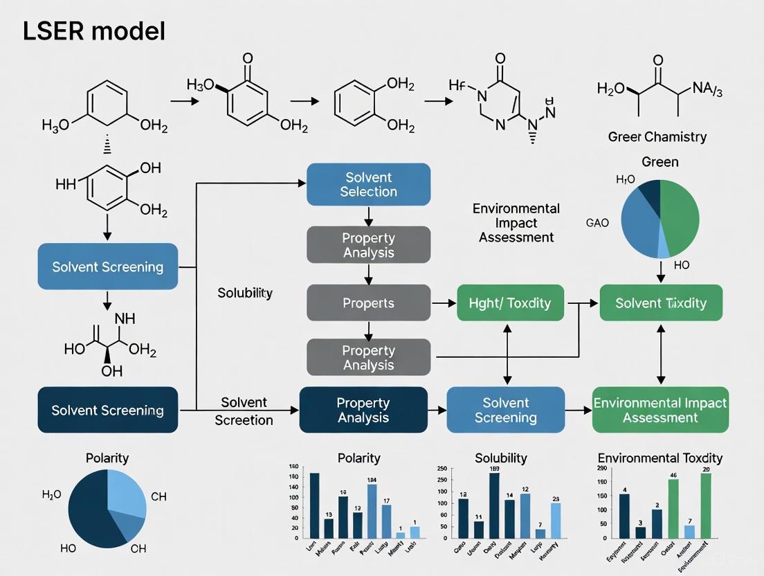
LSER Application Workflow in Solvent Screening
The following diagram illustrates the logical workflow for applying LSERs in a rational solvent screening methodology, from initial compound characterization to final solvent selection.
LSER-Based Solvent Screening Workflow
Data Presentation and Analysis
The predictive power of the LSER model is demonstrated by its application to diverse solvation-related properties. The following table summarizes representative LSER equations and coefficients for key properties relevant to pharmaceutical and chemical research. These equations allow for the quantitative prediction of a property for a new solute once its five descriptors are known.
Table 3: LSER Equations for Key Solvation Properties
| System / Property | LSER Equation | Notes & Application Context |
|---|---|---|
| n-Octanol/Water Partition Coefficient (Log K_ow) | Log K_ow = 0.43 + 5.35Vx - 0.43E - 3.60S - 0.22A - 4.27B | The negative coefficients for A and B show H-bonding disfavors partitioning into octanol from water. Crucial for predicting drug lipophilicity. |
| Water Solubility (Log S_w) | Log S_w = 0.43 - 5.35Vx + 0.43E + 3.60S + 0.22A + 4.27B | Essentially the inverse of the Log K_ow LSER. H-bonding (A, B) and polarity (S) strongly favor aqueous solubility. |
| Gas/Hexadecane Partition Coefficient (Log L_HD) | Log L_HD = 0.23 + 6.89Vx + 1.13E + 0.47S + 2.15A + 4.12B | Models dispersion (Vx) and H-bonding (A, B) interactions with an inert alkane phase. Useful for GC retention prediction. |
| Dermal Permeability (Log K_p) | Log K_p = -1.26 + 4.12Vx - 0.56E - 2.12S - 3.60A - 4.78B | Highlights that large, non-polar, non-H-bonding molecules permeate skin more easily. Critical for transdermal drug design. |
Advanced Applications and Protocol for Predicting Partition Coefficients
Protocol: Predicting n-Octanol/Water Partition Coefficients (Log P)
Objective: To computationally predict the Log P value of a new chemical entity using its LSER descriptors and a pre-established LSER equation.
Materials:
- LSER descriptors for the target solute (Vx, E, S, A, B)
- Validated LSER equation for Log P (e.g., from Table 3)
- Computational tool (spreadsheet software or scripting environment)
Procedure:
- Descriptor Acquisition: Obtain or calculate the five LSER descriptors for the target solute. Vx can be calculated from structure using group contribution methods. E, S, A, and B can be determined experimentally (as per Protocol 3.1 and 3.2) or predicted using specialized software/QSPR models.
- Equation Application: Substitute the descriptor values into the validated LSER equation for Log P. For example, using the standard equation: Log P = 0.43 + 5.35Vx - 0.43E - 3.60S - 0.22A - 4.27B.
- Calculation: Perform the arithmetic calculation to obtain the predicted Log P value.
- Validation: Where possible, compare the predicted value with experimental data from the literature or a limited set of laboratory measurements to confirm the reliability of the prediction for the chemical space of interest.
Application in Drug Development: This protocol allows for the high-throughput screening of virtual compound libraries for their lipophilicity, a key parameter in the Rule of Five and other ADMET (Absorption, Distribution, Metabolism, Excretion, and Toxicity) prediction models. By understanding the specific contributions of volume, polarity, and hydrogen-bonding, medicinal chemists can make rational structural modifications to optimize a compound's partition behavior.
Integration with Modern Solvent Selection Tools
The LSER framework is increasingly integrated into sophisticated solvent selection and computer-aided molecular design (CAMD) tools. In these platforms, the LSER model serves as a fundamental physical property predictor. The workflow involves defining property constraints (e.g., a target Log P range or a minimum solubility) and then using the LSER equations to screen a vast database of solvents or solute molecules to identify candidates that meet the criteria. This represents the pinnacle of applying the core Vx, E, S, A, and B descriptors, moving from descriptive analysis to generative design in solvent screening methodology.
Linear Solvation Energy Relationships (LSERs) are a powerful quantitative tool used to understand and predict the partitioning behavior of solutes in different phases. At the heart of the Abraham solvation parameter model, the most widely used LSER formalism, lies a multiparameter equation that correlates a free-energy related property of a solute to its molecular descriptors [3] [4]. The most recent, widely accepted symbolic representation of this model is given by:
SP = c + eE + sS + aA + bB + vV
In this equation, SP is the solute property of interest, most often the logarithm of the retention factor in chromatography (log k') or the logarithm of a partition coefficient (log P) [3]. The capital letters (E, S, A, B, V) represent the solute's intrinsic molecular descriptors, while the lower-case letters (c, e, s, a, b, v) are the solvent system coefficients (also known as the system parameters or LFER coefficients) [4]. These coefficients are the focus of this application note. They are determined through a multiparameter linear least squares regression analysis of a data set comprised of solutes with known descriptor values [3]. Critically, these coefficients are solvent (phase or system) descriptors and are not influenced by the solute [4]. They are considered to correspond to the complementary effect of the phase (solvent) on solute-solvent interactions and contain chemical information on the solvent/phase in question [4].
Chemical Interpretation of the System Coefficients
The solvent system coefficients quantify the capability of the solvent system to engage in specific intermolecular interactions with the solute. The chemical interpretation of each coefficient is as follows:
c (The Constant Term): This is the regression equation intercept. Its value can represent the system property when all other interaction terms are zero, but its specific physicochemical meaning is not as straightforward as the other coefficients [5].
e (The Excess Polarizability Coefficient): This coefficient reflects the system's capacity to interact with solute n- or π-electrons, which contributes to the process of polarizability-dependent interactions [3] [4]. A positive 'e' value indicates that the process is favorable for polarizable solutes.
s (The Dipolarity/Polarizability Coefficient): This coefficient measures the system's ability to participate in dipole-dipole and dipole-induced dipole interactions with the solute [3]. A positive 's' value signifies that the system is more favorable for polar solutes.
a (The Hydrogen-Bond Basicity Coefficient): This coefficient characterizes the system's hydrogen bond accepting basicity (or proton accepting ability) [3] [4]. It describes the system's complementary ability to interact with a hydrogen-bond donor solute. A positive 'a' value means the system is a good H-bond acceptor and will strongly retain or dissolve solutes that are strong H-bond donors (high A).
b (The Hydrogen-Bond Acidity Coefficient): This coefficient characterizes the system's hydrogen bond donating acidity (or proton donating ability) [3] [4]. It describes the system's complementary ability to interact with a hydrogen-bond acceptor solute. A positive 'b' value means the system is a good H-bond donor and will strongly retain or dissolve solutes that are strong H-bond acceptors (high B).
v (The Cavity Formation Coefficient): This coefficient, also sometimes denoted as 'l' (L) in gas-to-solvent equations, represents the endoergic energy cost of forming a cavity in the solvent to accommodate the solute, as well as the dispersion interactions that occur upon insertion of the solute into that cavity [3] [4] [5]. It is strongly related to the solute's size (characteristic volume Vx). A positive 'v' value often indicates that cavity formation is the dominant process, which is typical in aqueous systems, while a negative value can indicate that dispersion interactions are more significant [3].
Table 1: Summary of LSER Solvent System Coefficients and Their Chemical Meanings
| Coefficient | Interaction it Represents | Probe Solute Property | Typical Interpretation |
|---|---|---|---|
| c | Constant | - | Regression intercept; system-dependent constant. |
| e | Polarizability | E (Excess molar refraction) | System's capacity for polarizability-based interactions. |
| s | Dipolarity/Polarizability | S (Dipolarity/Polarizability) | System's capacity for dipole-dipole interactions. |
| a | H-Bond Basicity | A (H-Bond Acidity) | System's complementary H-bond accepting ability. |
| b | H-Bond Acidity | B (H-Bond Basicity) | System's complementary H-bond donating ability. |
| v | Cavity Formation/Dispersion | V (McGowan Characteristic Volume) | System's resistance to cavity formation / strength of dispersion interactions. |
Quantitative Examples of System Coefficients
The values of the solvent system coefficients vary significantly between different partitioning systems, reflecting their unique chemical environments. The following table compiles published coefficients for several systems to illustrate their quantitative ranges and signs.
Table 2: Exemplary LSER System Coefficients for Different Partitioning Systems
| Partitioning System | c | e | s | a | b | v | Source / Reference |
|---|---|---|---|---|---|---|---|
| Low-Density Polyethylene / Water [5] | -0.529 | 1.098 | -1.557 | -2.991 | -4.617 | 3.886 | Egert et al. (2022) |
| Amorphous LDPE / Water [5] | -0.079 | - | - | - | - | - | Egert et al. (2022) |
| n-Hexadecane / Water (implied comparison) [5] | - | - | - | - | - | - | Egert et al. (2022) |
Interpretation of Examples:
- The LDPE/Water system shows a large positive v-coefficient, indicating that cavity formation in the aqueous phase is a major driving force, and solutes are partitioned into the polymer based largely on their size [5].
- The strongly negative a and b coefficients reveal that the LDPE/Water system is unfavorable for hydrogen-bonding interactions. A solute with strong H-bond donating (high A) or accepting (high B) ability will prefer the aqueous phase, leading to a lower partition coefficient into LDPE [5].
- The positive e coefficient suggests a slight favoring of polarizable solutes by the LDPE phase.
- The adjustment of the c-constant from -0.529 to -0.079 when considering the amorphous volume of LDPE demonstrates how the physical interpretation of the system can affect the coefficients, bringing it closer to a liquid-like partitioning system such as n-hexadecane/water [5].
Experimental Protocol for Determining System Coefficients
The following section provides a detailed methodology for determining the solvent system coefficients for a new two-phase partitioning system.
Materials and Equipment
Table 3: Research Reagent Solutions and Essential Materials
| Item / Reagent | Function / Specification |
|---|---|
| Probe Solute Set | A minimum of 20-30 structurally diverse, neutral compounds with known and well-established Abraham solute descriptors (E, S, A, B, V). The set should span a wide range of interaction abilities [3]. |
| Solvent System | The two phases of interest (e.g., organic solvent/water, polymer/water). Must be pure and of analytical grade. |
| Chromatography System | HPLC or GC system for measuring retention factors (log k'), if applicable. |
| Shaking Incubator | For thermostatted liquid-liquid partitioning experiments. |
| Analytical Instrumentation | HPLC-UV, GC-FID, or LC-MS for quantitative analysis of solute concentrations in both phases. |
| UFZ-LSER Database | A curated, free, web-based database to retrieve established solute descriptors for the probe solutes [6] [5]. |
Step-by-Step Workflow
The logical workflow for a typical LSER system characterization study is outlined in the diagram below. This protocol assumes a liquid-liquid partitioning experiment.
Detailed Experimental Procedures
Selection of Probe Solutes
Curate a training set of 20-30 neutral compounds. The selection is critical and must include solutes with a wide range of hydrogen-bond donor (A) and acceptor (B) abilities, dipolarity/polarizability (S), and size (V) [3]. Avoid congeneric series that lack diversity.
Measurement of Partition Coefficients (Log P)
For each probe solute, the partition coefficient between the two phases must be experimentally determined.
- Preparation: Prepare a saturated solution of the solute in one phase (e.g., the aqueous phase). For liquid-liquid systems, pre-saturate the immiscible solvents with each other to prevent volume changes.
- Equilibration: Combine equal volumes of the two phases in a sealed vial. Place the vial in a thermostatted shaking incubator (e.g., 25°C) and agitate for a sufficient time to reach equilibrium (typically 24-48 hours).
- Separation: After equilibration and settling, carefully separate the two phases.
- Analysis: Quantify the concentration of the solute in each phase using a suitable analytical method (e.g., HPLC-UV). The partition coefficient is calculated as P = Cₚₕₐₛₑ₂ / Cₚₕₐₛₑ₁, and the solute property becomes SP = log P.
Data Retrieval and Regression Analysis
- Descriptor Retrieval: For each probe solute in the training set, retrieve its Abraham solute descriptors (E, S, A, B, V) from a curated database such as the UFZ-LSER database [6].
- Multiple Linear Regression (MLR): Input the data (log P values and the five solute descriptors for all solutes) into statistical software capable of MLR. Perform regression analysis with log P as the dependent variable and E, S, A, B, V as the independent variables.
- Coefficient Extraction: The output of the MLR will provide the best-fit values for the system coefficients c, e, s, a, b, v, completing the LSER model for your specific partitioning system.
Model Validation and Best Practices
- Statistical Checks: Ensure the regression has a high coefficient of determination (R² > 0.95 is often achievable) and low root-mean-square error (RMSE) [5].
- Internal Validation: Use a portion of your data (~25-30%) as a validation set not used in the regression to test the model's predictive power [5].
- Chemical Sense: Evaluate the signs and magnitudes of the coefficients for chemical reasonableness. For instance, an aqueous phase should have positive a and b coefficients (strong H-bonding ability) and a positive v coefficient (significant cavity term) [3].
- Advisories: As recommended by Vitha et al., always report the standard errors of the coefficients, the list of solutes used, and the statistical parameters of the regression to ensure the transparency and reproducibility of your LSER study [3].
Application in Solvent Screening and Pharmaceutical Research
The derived LSER model with its system coefficients is a powerful tool for predictive solvent screening. In pharmaceutical development, it can be used to:
- Predict Partitioning: For a new drug compound with known or predicted solute descriptors, its log P for the characterized system can be calculated directly using the LSER equation, bypassing laborious experiments [5] [7].
- Understand Formulation Behavior: The model provides a mechanistic understanding of how a drug will distribute in complex systems, which is crucial for optimizing drug delivery, bioavailability, and extraction processes [8] [9] [10].
- Benchmark Polymers: As shown in Table 2, LSERs allow for the direct comparison of different polymeric materials (e.g., LDPE, PDMS, Polyacrylate) as sorbents based on their system parameters, guiding the selection of materials with desired interaction properties [5].
By following the protocols outlined in this document, researchers can robustly characterize solvent systems and leverage the rich chemical information encoded in the 'c', 'e', 's', 'a', 'b', and 'v' parameters to advance their solvent screening and product development pipelines.
The Abraham Solvation Parameter Model, more commonly known as the Linear Solvation Energy Relationship (LSER), represents one of the most successful predictive frameworks in molecular thermodynamics for characterizing solute-solvent interactions [4]. This model provides a quantitative bridge between molecular structure and thermodynamic behavior through linear free energy relationships, enabling researchers to predict partitioning, solvation, and chromatographic retention properties across diverse chemical systems. The fundamental premise of LSER lies in its ability to decompose complex solvation phenomena into discrete, physically meaningful molecular interactions, offering unparalleled utility in pharmaceutical research, environmental chemistry, and solvent screening methodologies [4] [11].
At its core, LSER formalizes the thermodynamic principle that free energy changes associated with solute transfer between phases correlate linearly with molecular descriptors that encapsulate specific interaction capabilities [4]. This linear free energy relationship (LFER) principle manifests practically through two primary equations that quantify solute partitioning between condensed phases and between gas-liquid systems, respectively. The robust thermodynamic foundation of LSER enables researchers to extract valuable information about intermolecular interactions from accessible experimental data, making it particularly valuable for drug development professionals who must predict compound behavior across biological membranes and formulation matrices [4] [12].
Theoretical Framework: LSER Equations and Molecular Descriptors
Fundamental LSER Equations
The LSER model operates through two principal equations that describe solute partitioning behavior in different thermodynamic contexts. For solute transfer between two condensed phases, the model employs:
log(P) = cp + epE + spS + apA + bpB + vpVx [4]
Where P represents the water-to-organic solvent or alkane-to-polar organic solvent partition coefficient. For gas-to-solvent partitioning, the relationship becomes:
log(KS) = ck + ekE + skS + akA + bkB + lkL [4]
Where KS denotes the gas-to-organic solvent partition coefficient. These linear relationships extend beyond free energy to encompass enthalpy changes during solvation:
ΔHS = cH + eHE + sHS + aHA + bHB + lHL [4]
This enthalpy relationship provides crucial insights into the energetic components of molecular interactions, complementing the free-energy perspective offered by the partition equations.
Molecular Descriptors and their Physical Significance
The LSER model characterizes each solute through six fundamental molecular descriptors that capture distinct aspects of its interaction potential:
Table 1: LSER Molecular Descriptors and Their Thermodynamic Interpretation
| Descriptor | Symbol | Physical Interpretation | Thermodynamic Basis |
|---|---|---|---|
| McGowan's Characteristic Volume | Vx | Molecular size and cavity formation energy | Measures work required to create a cavity in solvent |
| Gas-Hexadecane Partition Coefficient | L | Dispersion interactions and molecular polarizability | Reflects London dispersion forces with n-alkane reference |
| Excess Molar Refraction | E | Polarizability from n- and π-electrons | Captures interactions with solute polarizability |
| Dipolarity/Polarizability | S | Dipole-dipole and dipole-induced dipole interactions | Represents Keesom and Debye forces |
| Hydrogen Bond Acidity | A | Hydrogen bond donating ability | Quantifies solute ability to donate protons |
| Hydrogen Bond Basicity | B | Hydrogen bond accepting ability | Quantifies solute ability to accept protons |
The lower-case coefficients in the LSER equations (ep, sp, ap, bp, vp, etc.) represent complementary solvent properties that characterize the phase or solvent system [4]. These are determined through multilinear regression of experimental data and remain specific to each solvent system while being independent of the solute, forming the basis for the model's predictive capability across diverse molecular structures.
Thermodynamic Basis of LSER Linearity
Free Energy Relationships and Molecular Interactions
The remarkable linearity observed in LSER relationships, even for strong specific interactions like hydrogen bonding, finds its foundation in the fundamental principles of solution thermodynamics [4]. The LSER model successfully operates because the Gibbs free energy of solvation (ΔGsolv) can be separated into additive contributions from distinct intermolecular interaction types, with each contribution proportional to the product of a solute-specific descriptor and its complementary solvent-specific coefficient [4] [12]. This additivity principle emerges from the mathematical structure of solution thermodynamics when applied to transfer processes between phases with different interaction potentials.
The hydrogen-bonding terms (apA + bpB) in the LSER equations deserve particular attention, as they quantify the strong specific interactions that often dominate solvation thermodynamics in pharmaceutical and biological systems [4]. The linearity of these terms persists because hydrogen bonding contributions to free energy remain approximately proportional to the product of donor and acceptor capabilities across a wide range of chemical space, though deviations can occur in systems with strong cooperativity or intramolecular hydrogen bonding [12]. This linear approximation holds practical value for solvent screening despite its theoretical limitations in extreme cases.
Connecting LSER to Equation-of-State Thermodynamics
Recent advances have focused on bridging the LSER framework with equation-of-state thermodynamics through the development of Partial Solvation Parameters (PSP) [4]. This integration aims to extract the rich thermodynamic information embedded in LSER databases for broader applications in molecular thermodynamics. The PSP approach defines four key parameters that mirror the LSER interaction domains: hydrogen-bonding acidity (σa), hydrogen-bonding basicity (σb), dispersion (σd), and polar (σp) interactions [4].
The interconnection between LSER and PSP frameworks enables researchers to transform LSER molecular descriptors into thermodynamic properties relevant for equation-of-state calculations, including the free energy change (ΔGhb), enthalpy change (ΔHhb), and entropy change (ΔShb) associated with hydrogen bond formation [4]. This connection provides a pathway to extend LSER predictions beyond partition coefficients to include temperature-dependent properties and phase equilibria, significantly expanding the model's utility in pharmaceutical process development.
Experimental Protocols for LSER Parameterization
Chromatographic Determination of LSER Descriptors
Liquid chromatography provides an efficient experimental platform for determining LSER parameters for novel compounds. The following protocol outlines a streamlined approach for characterizing solute-solvent interactions in reversed-phase and HILIC systems:
Table 2: Experimental Protocol for LSER Parameter Determination via Chromatography
| Step | Procedure | Purpose | Critical Parameters |
|---|---|---|---|
| 1. Column Conditioning | Equilibrate column with mobile phase (e.g., water-acetonitrile gradient) | Ensure reproducible stationary phase properties | Flow rate: 1.0 mL/min; Temperature: 25°C |
| 2. Hold-up Volume Determination | Inject four alkyl ketone homologues (C3-C6) | Establish column dead time (t0) for retention factor calculation | Detection: UV at 254 nm; Injection volume: 5 μL |
| 3. Test Compound Analysis | Inject carefully selected solute pairs with differing single descriptors | Isolate specific solute-solvent interactions | Minimum duplicate injections; Randomize injection order |
| 4. Retention Factor Calculation | Calculate k = (tR - t0)/t0 for all compounds | Normalize retention data for LSER analysis | Use average retention times from replicates |
| 5. Selectivity Factor Determination | Calculate α = k2/k1 for solute pairs | Quantify contribution of specific molecular interactions | Pair compounds with similar descriptors except one |
| 6. LSER Regression | Perform multilinear regression of log k against descriptors | Obtain system-specific LSER coefficients | Minimum 15-20 test solutes for reliable regression |
This protocol enables complete characterization of a chromatographic system with just five experimental runs (four solute pairs and one homologue mixture), significantly enhancing throughput compared to traditional LSER approaches that require 30-40 test solutes [11]. The strategic selection of solute pairs that differ in only one molecular descriptor allows researchers to deconvolute the individual contributions of cavity formation, dispersion, polarity, and hydrogen bonding to the overall retention mechanism.
Determination of Solvation Enthalpies
For thermodynamic profiling beyond partition coefficients, the following protocol enables determination of solvation enthalpies compatible with LSER analysis:
Calorimetric Measurement: Utilize isothermal titration calorimetry (ITC) or solution calorimetry to measure enthalpy changes associated with solute transfer from gas to solvent or between liquid phases.
Temperature Variation Studies: Conduct partitioning or chromatographic experiments at multiple temperatures (typically 3-5 points between 15-35°C) to derive enthalpy values from van't Hoff analysis.
Data Regression: Apply the LSER enthalpy equation (ΔHS = cH + eHE + sHS + aHA + bHB + lHL) to the experimental data using multilinear regression to obtain the enthalpy-specific system coefficients [4].
Cross-Validation: Compare LSER-predicted enthalpies with experimental values for validation compounds not included in the regression set.
This approach provides direct access to the enthalpic components of molecular interactions, offering deeper insights into the nature and strength of solute-solvent interactions beyond what can be learned from partition coefficients alone.
Research Reagent Solutions for LSER Studies
Table 3: Essential Research Reagents for LSER Experimental Characterization
| Reagent Category | Specific Examples | Function in LSER Studies |
|---|---|---|
| Reference Alkanes | n-Hexane, n-Heptane, n-Octane, n-Hexadecane | Characterization of dispersion interactions and cavity formation |
| Hydrogen-Bonding Probes | Phenol, p-Cresol, Aniline, Pyridine, N-Methylpyrrolidone | Quantification of hydrogen-bonding acidity and basicity |
| Polarity Standards | Nitrobenzene, Dimethyl sulfoxide, Acetone, Dichloroethane | Assessment of dipole-dipole and dipole-induced dipole interactions |
| Cavity Formation Markers | Alkylbenzenes, Polyaromatic hydrocarbons, Alkyl ketones | Measurement of molecular volume-dependent contributions |
| Chromatographic Columns | C18, Cyano, Phenyl, HILIC, Polar-embedded phases | Diverse stationary phases for interaction mapping |
| Mobile Phase Modifiers | Water, Acetonitrile, Methanol, Buffer systems | Mobile phase manipulation to modulate interaction strength |
The strategic selection and application of these research reagents enables comprehensive characterization of solute-solvent interactions across diverse chemical spaces. Particularly valuable are compound pairs that share similar molecular descriptors except for one specific interaction property, allowing researchers to isolate individual contribution to the overall solvation thermodynamics [11].
Visualization of LSER Concepts and Workflows
Thermodynamic Foundation of LSER Linearity
This diagram illustrates the conceptual workflow connecting molecular structure to thermodynamic properties through the LSER framework. The pathway begins with molecular characterization, proceeds through the application of LSER equations with appropriate solvent parameters, and culminates in the determination of free energy changes that can be deconvoluted into specific molecular interaction contributions.
Experimental Protocol for LSER Parameterization
This workflow details the experimental sequence for determining LSER parameters through chromatographic methods. The protocol emphasizes the importance of careful system calibration, strategic selection of analyte pairs with complementary descriptor profiles, and systematic data analysis to extract the system-specific coefficients that quantify different interaction types.
Applications in Solvent Screening and Pharmaceutical Development
The integration of LSER thermodynamics into solvent screening methodologies provides drug development professionals with powerful tools for predicting compound behavior across multiple contexts. In pharmaceutical applications, LSER enables a priori prediction of drug solubility, membrane permeability, and distribution coefficients without extensive experimental measurement [4] [11]. The model's ability to deconvolute the contributions of different interaction types to the overall solvation free energy allows researchers to rationally select formulation components that optimize solubility and stability while minimizing toxicity and production costs.
For solvent screening specifically, LSER coefficients facilitate systematic comparison of solvent properties and their compatibility with target solutes. By mapping solvents in a space defined by their hydrogen-bonding, polar, and dispersion interaction parameters, researchers can identify optimal solvent mixtures that maximize solvation power for specific compound classes. This approach significantly accelerates the solvent selection process in early-stage development while providing fundamental insights into the molecular interactions governing solute dissolution and crystallization behavior. The extension of LSER through Partial Solvation Parameters further enables predictions across temperature ranges, supporting the development of robust crystallization processes and thermodynamic models for pharmaceutical manufacturing.
Solvent selection is a critical determinant in the success of processes ranging from drug formulation to materials synthesis. While the Linear Solvation Energy Relationship (LSER) model provides a multi-parameter approach for predicting solute-solvent interactions, traditional polarity scales like Kamlet-Taft and Hansen Solubility Parameters (HSP) remain widely used for their conceptual simplicity and predictive power. This Application Note delineates the theoretical foundations, practical applications, and experimental protocols for these solvent characterization methods, providing researchers in drug development with a clear framework for selecting the optimal solvent screening methodology for their specific needs. The content is framed within a broader thesis on advancing solvent screening methodologies using the LSER model, highlighting its integrative capacity compared to other established parameter systems.
A comparative overview of these solvent parameter systems is provided in Table 1.
Table 1: Comparison of Major Solvent Parameter Systems
| Parameter System | Core Parameters | Molecular Interactions Described | Primary Application Context |
|---|---|---|---|
| LSER (Linear Solvation Energy Relationship) | π* (Polarity/Polarizability), α (H-bond Acidity), β (H-bond Basicity) | Dipolarity/polarizability, Hydrogen-bond donation (acidity), Hydrogen-bond acceptance (basicity) | Modeling complex solubility phenomena and reaction rates; correlating multiple solvent properties with biological activity [13] [14]. |
| Kamlet-Taft Solvatochromic Parameters | π* (Polarity/Polarizability), α (H-bond Acidity), β (H-bond Basidity) | Dipolarity/polarizability, Hydrogen-bond donation (acidity), Hydrogen-bond acceptance (basicity) | Solvatochromic analysis; pre-screening solvent effects on molecular probes and drug candidates [13] [14]. |
| Hansen Solubility Parameters (HSP) | δD (Dispersive), δP (Polar), δH (Hydrogen-bonding) | Dispersion forces, Permanent dipole-permanent dipole interactions, Hydrogen bonding | Predicting polymer solubility and gelation ability; mapping solvent space for formulation [14]. |
Theoretical Framework and Key Parameters
Linear Solvation Energy Relationship (LSER)
The LSER model quantitatively correlates a solute's property (e.g., solubility, reaction rate, biological activity) to a set of solvent parameters that describe different aspects of solvation. The general form of a LSER equation for a property SP is often expressed as:
SP = SP₀ + sπ* + aα + bβ
Here, SP₀ is the property value in a reference solvent, and the coefficients s, a, and b represent the sensitivity of the property to the solvent's polarizability (π*), hydrogen-bond acidity (α), and hydrogen-bond basicity (β), respectively [14]. The power of the LSER lies in its ability to deconvolute the individual contribution of each interaction type, providing deep mechanistic insight. For instance, it has been successfully used to model the solubility of pharmaceuticals like naphthalene and benzoic acid in various solvents by establishing a quantitative relationship between the measured Kamlet-Taft parameters of the solvents and the solubility data [13].
Kamlet-Taft Solvatochromic Parameters
The Kamlet-Taft parameters are empirically derived from the solvatochromic shifts of various dye probes, meaning they are based on how a solvent changes the color (UV-Vis absorption maxima) of these dyes.
- π* (Polarity/Polarizability): Measures the solvent's ability to stabilize a charge or a dipole through non-specific dielectric and polarization effects.
- α (Hydrogen-Bond Acidity): Quantifies the solvent's ability to donate a hydrogen bond.
- β (Hydrogen-Bond Basicity): Quantifies the solvent's ability to accept a hydrogen bond [13] [14].
These parameters are particularly valuable for understanding solvent effects on spectroscopic properties and reaction mechanisms involving excited states or polar intermediates.
Hansen Solubility Parameters (HSP)
Hansen Solubility Parameters (HSP) partition the total Hildebrand solubility parameter (δT) into three components representing distinct intermolecular forces:
- δD (Dispersive Interactions): Arises from London dispersion forces.
- δP (Polar Interactions): Results from permanent dipole-permanent dipole interactions.
- δH (Hydrogen-Bonding Interactions): Accounts for hydrogen bonding forces [14].
The solubility of a material in a solvent is predicted by calculating the Hansen distance (Ra) between the solute and solvent. A smaller Ra indicates greater solubility similarity. HSPs are extensively applied in polymer science and coatings, and are increasingly used for molecular gels. Research on the gelator DBS (1,3:2,4-dibenzylidene sorbitol) has shown that the hydrogen-bonding parameter (δH) is particularly critical, and the directionality of the difference in δH between solvent and solute can determine the optical clarity of the resulting gel [14].
Experimental Protocols
Determination of Kamlet-Taft Parameters via Solvatochromic Probes
This protocol details the experimental method for determining the Kamlet-Taft π*, α, and β parameters for a series of solvents, including hydrofluoroethers (HFEs) [13].
Research Reagent Solutions
Table 2: Essential Reagents for Kamlet-Taft Parameter Determination
| Item | Function/Description | Critical Notes |
|---|---|---|
| Solvatochromic Probes | Reichardt's dye, N,N-diethyl-4-nitroaniline, 4-nitroanisole, etc. | Probes are selected for their specific sensitivity to π*, α, or β. Must be of high purity. |
| Anhydrous Solvents | Hydrofluoroethers (HFEs), other target solvents. | Solvents must be purified to remove water and impurities that could affect H-bonding. |
| UV-Vis Spectrophotometer | Measures electronic transition maxima (absorption peaks). | Requires temperature control for thermosolvatochromic studies [13]. |
| Quartz Cuvettes | Holds liquid sample for spectroscopic analysis. | Must be sealed for volatile solvents or elevated temperature studies. |
Step-by-Step Procedure
- Solution Preparation: Prepare solutions of each solvatochromic probe in the anhydrous solvent of interest at a concentration suitable for UV-Vis spectroscopy (typically ensuring absorbance maxima are within the instrument's linear range).
- Spectroscopic Measurement: Place the solution in a temperature-controlled quartz cuvette. Record the UV-Vis absorption spectrum across the appropriate wavelength range (e.g., 300-800 nm, depending on the probe) at a defined temperature.
- Data Acquisition: Precisely determine the wavelength of the maximum absorption (λmax) for each probe in each solvent. Repeat measurements at different temperatures to obtain thermosolvatochromic data if required [13].
- Parameter Calculation: Calculate the Kamlet-Taft parameters using the established empirical equations and the measured λmax values. For example, the solvent polarity π* is often derived from the shift of 4-nitroanisole, while α and β are calculated from probes like Reichardt's dye and nitroanilines, respectively [13] [14].
The workflow for this protocol is systematized in the diagram below.
Hansen Solubility Parameters and Gelation Testing
This protocol, adapted from studies on molecular gelators like DBS, describes how to determine a solvent's gelation ability and correlate it with its HSP values [14].
Research Reagent Solutions
Table 3: Essential Reagents for Gelation Testing and HSP Correlation
| Item | Function/Description | Critical Notes |
|---|---|---|
| Molecular Gelator | e.g., DBS (1,3:2,4-dibenzylidene sorbitol) | A well-characterized gelator for method validation. |
| Solvent Library | A diverse set of solvents covering a wide range of δD, δP, δH values. | Essential for building a robust correlation [14]. |
| Heating Block with Vials | For dissolving the gelator in solvents at elevated temperatures. | Vials should be sealed with Teflon liners to prevent solvent evaporation. |
| Rheometer | Characterizes mechanical properties (G', G'') of the formed gel. | Optional but recommended for quantitative gel strength analysis. |
Step-by-Step Procedure
- Sample Preparation: Add a known amount of the gelator (e.g., 1-5 wt%) to a solvent in a sealed vial. Heat the mixture in a heating block until a clear, persistent solution is obtained (e.g., 5 minutes at a temperature above the gelator's dissolution point).
- Gelation Incubation: Cool the vial to the test temperature (e.g., room temperature or a controlled 20°C or 40°C for higher-melting solvents) and incubate for a standardized period (e.g., 24 hours) [14].
- Inversion Test: Qualitatively assess gelation by inverting the vial for a set time (e.g., 1 hour). Classify the sample as a "sol" (flow is observed), a "gel" (no flow), and note the optical clarity ("clear gel" or "opaque gel") [14].
- Data Correlation: Plot the results (sol, clear gel, opaque gel) in 3D Hansen space or 2D projections. Analyze the clustering of successful gelation regions relative to the HSP coordinates of the solvents and the gelator. The directionality of the hydrogen-bonding parameter (δh) difference between solvent and gelator can be a critical factor [14].
The logical flow for correlating solvent properties with gelation outcomes is as follows.
Data Presentation and Analysis
The quantitative data derived from these protocols must be structured for clear comparison and model building. Below are examples of how to present key data.
Table 4: Exemplar Data Table for Solvent Parameters and Observed Properties (Adapted from [13] [14])
| Solvent | Kamlet-Taft Parameters | Hansen Solubility Parameters (MPa^1/2) | Observed Property | ||||||
|---|---|---|---|---|---|---|---|---|---|
| π* | α | β | δD | δP | δH | Log P | Naphthalene Solubility (LSER) | DBS Gelation Outcome | |
| HFE-7100 | 0.47 | 0.00 | 0.12 | - | - | - | - | Modeled by LSER [13] | - |
| 1-Butanol | ~0.4 | ~0.8 | ~0.9 | 16.0 | 5.7 | 15.8 | ~0.8 | - | Sol [14] |
| 3-Pentanone | ~0.7 | ~0.0 | ~0.5 | 15.8 | 7.0 | 5.0 | ~0.8 | - | Clear Gel [14] |
Integrated Application in Solvent Screening
For a comprehensive solvent screening methodology in drug development, the strengths of each parameter system can be leveraged in an integrated workflow. The LSER model serves as the overarching framework for building quantitative predictive models for complex properties like drug solubility or permeability. The required Kamlet-Taft or Hansen parameters for new solvents can be determined experimentally or sourced from literature.
This integrated approach allows researchers to move beyond simplistic "like-dissolves-like" rules. For instance, as demonstrated in Table 4, 1-butanol and 3-pentanone have similar relative permittivities and log P values, yet they exhibit dramatically different behaviors with the gelator DBS. This difference is captured by their distinct hydrogen-bonding profiles (high α and δH for 1-butanol vs. low α and δH for 3-pentanone), a nuance that is critical for formulation and is effectively highlighted by Kamlet-Taft and Hansen parameters, and can be incorporated into a robust LSER model [14].
Implementing LSER: A Step-by-Step Methodology for Solvent Screening
The challenge of poor water solubility affects a significant proportion of traditional drugs and approximately 90% of new chemical entities (NCEs), presenting a major hurdle in pharmaceutical development [15]. Linear Solvation Energy Relationship (LSER) models have emerged as powerful in silico tools for predicting and improving solute solubility, offering a systematic methodology for solvent screening that can significantly reduce the need for extensive experimental trials [15] [16]. This application note provides a detailed protocol for implementing LSER-based solubility prediction, framed within a comprehensive solvent screening methodology for pharmaceutical applications. We present a structured workflow from molecular structure analysis to quantitative solubility prediction, enabling researchers to efficiently identify optimal solubilization strategies for poorly soluble drug compounds.
Theoretical Foundation of LSER Models
LSER models are based on the principle that solvation properties can be correlated with fundamental molecular descriptors through multi-parameter linear equations [17] [4]. The Abraham solvation parameter model, a widely implemented LSER approach, correlates free-energy-related properties of a solute with its six molecular descriptors: McGowan's characteristic volume (Vx), the gas-liquid partition coefficient in n-hexadecane (L), excess molar refraction (E), dipolarity/polarizability (S), hydrogen bond acidity (A), and hydrogen bond basicity (B) [4].
For solubility prediction, the LSER framework can be expressed as:
log S = c + eE + sS + aA + bB + vVx
Where S represents the solubility of the molecule, and the lower-case coefficients (e, s, a, b, v) are system descriptors that reflect the complementary effect of the solvent phase on solute-solvent interactions [15] [4]. The constant c represents a system-specific intercept. This linear relationship holds across diverse chemical systems due to its foundation in solvation thermodynamics, even accounting for strong specific interactions such as hydrogen bonding [4].
Experimental and Computational Workflow
The following section outlines a comprehensive protocol for applying LSER methodology to solubility prediction, integrating both computational and experimental components.
The diagram below illustrates the integrated workflow from molecular structure to solubility prediction:
Molecular Descriptor Determination
Quantum Chemical Calculations
Protocol: Density Functional Theory (DFT) Optimization
- Input Preparation: Generate initial 3D molecular structures for both solute and solvent molecules using chemical drawing software or structure generators.
- Geometry Optimization: Perform DFT calculations using functionals such as B3LYP with basis sets like 6-31G(d) to obtain optimized molecular geometries.
- Electronic Property Calculation: Compute electronic properties including highest occupied molecular orbital (HOMO) and lowest unoccupied molecular orbital (LUMO) energies, electronegativity (χ), and polarity indices from the optimized structures [15].
- COSMO-RS Implementation: For solvents, employ COSMO-RS (Conductor-like Screening Model for Real Solvents) to compute σ-profiles and σ-potentials, which provide theoretical descriptors for quantifying solvent effects [16].
Experimental Descriptor Determination
Protocol: Experimental Parameter Measurement
- Partition Coefficient (log P) Determination:
- Prepare n-octanol and water phases saturated with each other
- Dissolve solute in pre-saturated n-octanol phase
- Equilibrate equal volumes of n-octanol and water phases with solute
- Separate phases and quantify solute concentration in each phase using HPLC or UV-Vis spectroscopy
- Calculate log P = log(Coctanol/Cwater)
- Hydrogen Bonding Parameter Determination:
- Characterize hydrogen bond acidity (A) and basicity (B) through solvatochromic measurements using indicator dyes
- Alternatively, calculate from theoretical parameters derived from DFT calculations
LSER Model Development and Application
Protocol: Model Building and Validation
- Data Set Compilation: Collect experimental solubility data for a diverse set of reference compounds in the target solvent system. For drug solubility with cucurbit[7]uril, relevant data may include values such as:
Table 1: Experimental solubility data for selected drugs with cucurbit[7]uril in water [15]
| Drug | S (g L⁻¹) | S (μM) | log S (μM) |
|---|---|---|---|
| Cinnarizine | 5.049 | 13,700.000 | 4.137 |
| Allopurinol | 1.200 | 8,816.000 | 3.945 |
| Gefitinib | 1.734 | 3,880.891 | 3.589 |
| Triamterene | 0.923 | 3,643.070 | 3.561 |
| Vitamin B2 | 0.353 | 937.862 | 2.972 |
| Camptothecin | 0.139 | 400.000 | 2.602 |
| Cholesterol | 0.017 | 45.000 | 1.653 |
- Descriptor Matrix Construction: Compile molecular descriptors for all compounds in the data set.
- Model Parameterization: Perform multiple linear regression analysis to determine system-specific coefficients (e, s, a, b, v, c) using the equation provided in Section 2.
- Model Validation: Validate the model using an independent test set of compounds not included in the training set. For robust prediction, the model should achieve R² > 0.98 and RMSE < 0.35 for log solubility values [17].
Solubility Prediction Protocol
Protocol: Application of LSER Model for New Compounds
- Descriptor Calculation: Determine molecular descriptors for the new compound using the methods described in Section 3.2.
- Model Application: Input the molecular descriptors into the parameterized LSER model to predict solubility.
- Statistical Assessment: Calculate prediction intervals to quantify uncertainty in the solubility estimate.
- Solvent Screening: Apply the model across multiple solvent systems to identify optimal solubilization conditions.
Pharmaceutical Case Study: Cucurbit[7]uril as Solubilizing Agent
To illustrate the practical application of this workflow, we present a case study on predicting drug solubility with cucurbit[7]uril, a macrocyclic host molecule with high binding constants (up to 10¹⁵ M⁻¹ in water) and excellent stability in acidic and alkaline conditions [15].
Experimental Methods for Solubility Determination
Protocol: Equilibrium Solubility Measurement with Cucurbit[7]uril
- Sample Preparation:
- Add excess drug to 10 mL aqueous solutions containing varying concentrations of cucurbit[7]uril (0-15.0 mM)
- Vibrate samples for 1 hour on ultrasonic equipment
- Stir at room temperature in the dark until equilibrium is reached (24 hours)
- Analysis:
- Filter samples to remove undissolved drug
- Dilute filtrate with H₂O as needed
- Measure ultraviolet absorption at compound-specific wavelengths:
- Vitamin B₂ (VB₂): 446 nm
- Triamterene: 358 nm
- Guanine: 295 nm
- 2-hydroxychalcone: 323 nm
- Gefitinib: 335 nm
- Data Processing:
- Calculate solubility from calibration curves
- Express results as log S (μM) for LSER modeling
LSER Model Parameters for Cucurbit[7]uril System
The LSER model for drug solubility with cucurbit[7]uril identified several statistically significant parameters that influence solubilization [15]:
Table 2: Key parameters identified in LSER model for drug solubility with cucurbit[7]uril [15]
| Parameter | Molecular Interpretation | Significance in Solubilization |
|---|---|---|
| A₃ (Surface area of inclusion complexes) | Molecular size of the host-guest complex | Influences cavity formation energy and hydrophobic interactions |
| E₃LUMO (LUMO energy of inclusion complexes) | Electron acceptor capability | Affects charge transfer interactions and complex stability |
| I₃ (Polarity index of inclusion complexes) | Overall molecular polarity | Impacts solvation energy in aqueous medium |
| χ₁ (Electronegativity of drugs) | Electron withdrawing power | Influences hydrogen bonding capability and polar interactions |
| log P₁w (Oil-water partition coefficient of drugs) | Hydrophobicity/hydrophilicity balance | Determines baseline solubility in water |
Essential Research Reagents and Materials
The following table details key reagents and materials required for implementing the LSER solubility prediction workflow:
Table 3: Essential research reagents and materials for LSER solubility studies
| Reagent/Material | Function/Application | Examples/Specifications |
|---|---|---|
| Cucurbit[7]uril | Macrocyclic host for inclusion complexes | Purity >95%, aqueous solubility 20-30 mM [15] |
| Reference Drug Compounds | Model solutes for LSER parameterization | Cinnarizine, allopurinol, gefitinib, triamterene [15] |
| Deuterium-Depleted Water | Alternative solvent for solubility enhancement | ≤1 ppm D/H, modifies cluster structure and dissolution properties [18] |
| n-Octanol | Partition coefficient determination | HPLC grade, for log P measurements |
| Spectrophotometric Cuvettes | UV-Vis absorbance measurements | Quartz, 1 cm path length for solubility quantification |
| HPLC System | Compound quantification and purity assessment | Reverse-phase C18 columns, UV detector |
| Quantum Chemistry Software | Molecular descriptor calculation | COSMO-RS, DFT packages (Gaussian, ORCA) [16] |
This application note has detailed a comprehensive workflow for predicting solubility from molecular structure using LSER methodology. The integration of computational quantum chemistry with experimentally validated models provides a powerful framework for solvent screening in pharmaceutical development. The case study on cucurbit[7]uril illustrates how specific molecular interactions can be quantified and leveraged for solubility enhancement of poorly soluble drugs. By implementing this protocol, researchers can efficiently identify optimal formulation strategies, reducing the time and resources required for experimental screening while gaining fundamental insights into solute-solvent interactions.
Linear Solvation Energy Relationship (LSER) models are a fundamental pillar in modern solvent screening methodology. The predictive power of an LSER model is intrinsically tied to the quality and origin of the molecular descriptors it employs. These descriptors, such as hydrogen bond acidity (α), hydrogen bond basicity (β), and polarity/polarizability (π*), quantitatively capture the intermolecular interactions between a solute and its solvent environment [8]. The central challenge for researchers lies in selecting the optimal source for these critical parameters: should one use experimentally determined values or leverage the growing power of Quantitative Structure-Property Relationship (QSPR) prediction tools? This Application Note provides a detailed comparison of these two descriptor-sourcing paradigms and offers structured protocols for their application within LSER-driven solvent screening research.
Comparative Analysis: Experimental vs. QSPR-Based Descriptors
The choice between experimental and QSPR-sourced descriptors involves trade-offs between data reliability, availability, and resource expenditure. The following table summarizes the core characteristics of each approach.
Table 1: Comparison of Experimental and QSPR-Based Descriptor Sourcing
| Feature | Experimentally Sourced Descriptors | QSPR-Predicted Descriptors |
|---|---|---|
| Fundamental Principle | Direct measurement of solvatochromic effects or physicochemical properties in well-defined assays [8]. | Mathematical models correlating molecular structure (encoded by descriptors) with a target property [19] [20]. |
| Primary Advantage | High accuracy and direct empirical foundation; considered the "gold standard" [8]. | High-throughput; enables screening of novel, unsynthesized, or hazardous compounds [19] [20]. |
| Key Limitation | Data is limited to commercially available, stable, and pure compounds; time and resource-intensive [21]. | Predictive accuracy is contingent on model quality, training data, and applicability domain [22]. |
| Ideal Use Case | Final model validation and establishing benchmark relationships for key compound classes. | Rapid screening of large virtual chemical libraries and guiding the design of novel solvents [19]. |
| Resource Demand | High (specialized equipment, chemicals, analyst time). | Low to moderate (computational resources, software expertise). |
| Data Availability | Limited to known compounds. | Virtually unlimited for structures within the model's applicability domain. |
Protocols for Sourcing and Applying Descriptors in LSER Models
Protocol A: Utilizing Experimentally Derived LSER Descriptors
This protocol outlines the steps for building an LSER model using descriptors sourced from experimental literature or direct measurement.
A.1 Solvent Selection and Data Collection
- Identify a set of candidate solvents relevant to your separation process (e.g., methanol, ethanol, 2-propanol for aqueous mixtures) [8].
- Perform a systematic literature search for pre-existing LSER descriptors (α, β, π*, etc.) for the selected solvents. Reputable sources include peer-reviewed journals and curated physicochemical databases.
- Critical Step – Data Verification: Ensure that the experimental conditions (temperature, measurement technique) of the sourced descriptors are consistent across your dataset.
A.2 LSER Model Construction and Analysis
- Compile the experimental property data you wish to model (e.g., solute solubility) alongside the collected descriptors.
- Construct the LSER model using multiple linear regression (MLR), where the solute property is the dependent variable and the solvatochromic parameters are the independent variables [8].
- Analyze the regression coefficients to interpret the relative contribution of each type of intermolecular interaction (e.g., hydrogen bonding, polar interactions) to the overall solvent effect.
A.3 Case Study: Solubility of Pentaerythritol A study on the solubility of pentaerythritol in aqueous alcohol mixtures successfully employed this protocol. The model, of the form: Log(Solubility) = C₀ + C₁(π) + C₂(α) + C₃(β) + ... revealed that the polarity/polarizability (π) and hydrogen bond acidity (α) of the solvent mixtures were the primary factors influencing solubility, providing actionable insights for process optimization [8].
Protocol B: Employing QSPR-Predicted Descriptors and Properties
This protocol is designed for high-throughput screening where experimental data is scarce, using QSPR to predict both descriptors and final properties.
B.1 Dataset Curation and Molecular Representation
- Define a large, virtual library of candidate solvents (e.g., a combinatorial library of ionic liquid cations and anions) [19] [20].
- Represent each molecular structure in a machine-readable format, typically the Simplified Molecular Input Line Entry System (SMILES) [21] [23].
- Critical Step – Applicability Domain: Define the chemical space of your training data. Any prediction for a molecule falling outside this domain should be treated with caution [22].
B.2Descriptor Calculation and Model Application
- Use a QSPR software tool (e.g., QSPRpred, CORAL) to calculate molecular descriptors directly from the SMILES strings [23] [24]. These can be 2D/3D descriptors or latent representations from deep learning models.
- Input the calculated descriptors into a pre-validated QSPR model to predict the target property. Advanced deep learning frameworks like BERT-CNN-FNN can predict complex quantum chemical properties (e.g., σ-profiles) with high accuracy (R² > 0.97) directly from SMILES, bypassing the need for manual descriptor selection [21].
B.3 Case Study: Screening Ionic Liquids for Benzene Extraction Researchers developed QSPR models to screen ionic liquids for extracting benzene from fuels. Using a dataset of 112 ternary systems, they built both linear and non-linear (ANN) models linking 2D and 3D molecular descriptors of the ions to benzene distribution coefficients. The ANN model achieved excellent predictive accuracy (R² = 0.939), successfully identifying the anion size and electronegativity as key molecular features influencing extraction performance [19] [20].
Workflow Integration Diagram
The following diagram illustrates the logical relationship and integration points between the two descriptor-sourcing protocols within a comprehensive solvent screening research program.
The Scientist's Toolkit: Essential Research Reagent Solutions
Table 2: Key Software and Computational Tools for QSPR Modeling
| Tool Name | Type/Function | Key Application in Descriptor Sourcing |
|---|---|---|
| QSPRpred [24] | Open-Source Python Package | A flexible toolkit for building QSPR models, from data curation to model deployment. Supports multi-task learning. |
| CORAL-2023 [23] | QSPR Modeling Software | Uses SMILES notation and Monte Carlo optimization to build models and calculate correlation weight descriptors. |
| SMILES [21] [23] | Molecular Representation | The standard text-based representation for molecular structures, used as input for most modern QSPR and deep learning models. |
| Deep Learning Frameworks (e.g., BERT-CNN-FNN) [21] | Advanced ML Architecture | Captures complex molecular features directly from SMILES strings for end-to-end property prediction without manual descriptor selection. |
| VEGA [22] | QSAR Model Platform | Provides pre-built models for environmental property prediction (e.g., persistence, bioaccumulation). |
| EPI Suite [22] | Predictive Suite | Contains models like BIOWIN and KOWWIN for estimating physicochemical and environmental fate properties. |
Within the context of developing a robust solvent screening methodology, the Linear Solvation Energy Relationship (LSER) model stands as a powerful predictive tool for understanding and quantifying molecular interactions in chemical, environmental, and pharmaceutical systems [4]. Originally developed by Abraham, the LSER model provides a quantitative framework for correlating free-energy-related properties of solutes with molecular descriptors that encode specific interaction capabilities [3]. For researchers in drug development, this model offers invaluable insights into partitioning behavior, solubility, and other physicochemical properties critical to pharmaceutical optimization.
The fundamental premise of LSER is that any free-energy-related property (SP) can be correlated with a set of solute-specific parameters that represent a molecule's capacity for different types of intermolecular interactions [4] [3]. This approach has demonstrated remarkable success across various applications, from predicting environmental fate of chemicals to optimizing chromatographic separations and pharmaceutical formulations.
Core LSER Equations and Their Applications
The LSER framework utilizes two primary equations, each designed for specific phase transfer scenarios. Understanding the distinction between these equations is fundamental to implementing the model correctly.
The Partitioning Equation for Condensed Phases
For processes involving solute transfer between two condensed phases (e.g., water to organic solvent, blood to tissue), the following LSER equation applies [4]:
log(P) = cp + epE + spS + apA + bpB + vpVx
In this equation:
- P represents the partition coefficient between two condensed phases
- The lowercase coefficients (cp, ep, sp, ap, bp, vp) are system-specific constants that characterize the complementary properties of the phases between which partitioning occurs
- The uppercase variables (E, S, A, B, Vx) are solute-specific molecular descriptors
This equation is particularly valuable in pharmaceutical research for predicting tissue-blood distribution, skin permeability, and octanol-water partitioning (log P) - a key parameter in drug design [4].
The Gas-to-Solvent Partitioning Equation
For processes involving solute transfer from the gas phase to a condensed phase (e.g., air-to-water, air-to-blood), the appropriate LSER equation is [4]:
log(KS) = ck + ekE + skS + akA + bkB + lkL
In this equation:
- KS represents the gas-to-solvent partition coefficient
- The lowercase coefficients (ck, ek, sk, ak, bk, lk) describe the solvent phase
- The uppercase variables (E, S, A, B, L) are solute descriptors, with L replacing Vx as the size descriptor
This form is essential for predicting volatility, environmental distribution between air and biological fluids, and headspace concentrations in formulation studies.
Equation Selection Workflow
The following diagram illustrates the systematic process for selecting the appropriate LSER equation based on the system under investigation:
Molecular Descriptors and System Coefficients
The predictive power of LSER models stems from their foundation in well-defined molecular descriptors that quantify specific interaction capabilities.
Solute Descriptors (Independent Variables)
Table 1: LSER Solute Molecular Descriptors and Their Chemical Interpretation
| Descriptor | Chemical Interpretation | Measurement Basis | Range of Values |
|---|---|---|---|
| E | Excess molar refractivity | Polarizability from dispersion interactions | 0 to ~3.0 |
| S | Dipolarity/Polarizability | Ability to engage in dipole-dipole interactions | 0 to ~1.7 |
| A | Hydrogen bond acidity | Ability to donate a hydrogen bond | 0 to ~1.0 |
| B | Hydrogen bond basicity | Ability to accept a hydrogen bond | 0 to ~1.2 |
| Vx | McGowan's characteristic volume | Molecular size from van der Waals volume | ~0.2 to ~3.0 |
| L | Gas-hexadecane partition coefficient | Molecular size and dispersion interactions | -0.7 to ~8.0 |
These descriptors are determined experimentally through standardized measurements: Vx is calculated from molecular structure, L is obtained from gas-hexadecane partitioning at 298 K, E is derived from refractive index measurements, while S, A, and B are determined from various water-solvent partition coefficients and retention data [3].
System Coefficients (Fitted Parameters)
Table 2: LSER System Coefficients and Their Thermodynamic Meaning
| Coefficient | Chemical Interpretation | Represents Solvent/System's |
|---|---|---|
| e, c | Ability to engage in polarization interactions | Complementary polarizability |
| s, c | Dipolarity | Complementary dipolarity |
| a, c | Hydrogen bond basicity | Complementary hydrogen bond accepting ability |
| b, c | Hydrogen bond acidity | Complementary hydrogen bond donating ability |
| v, c | Cavity formation term | Energy cost of forming molecular-sized cavities |
| l, c | Dispersion interactions | Capacity for London dispersion forces |
The system coefficients are determined through multiple linear regression analysis of experimental data for a diverse set of solutes with known descriptors [4] [3]. These coefficients are temperature-dependent and fundamentally represent the difference in solvation properties between two phases [4].
Experimental Protocol for LSER Implementation
Phase I: System Definition and Data Collection
Define the partitioning system of interest based on your research question (e.g., blood-to-tissue distribution, water-to-membrane partitioning).
Select a diverse training set of 30-50 compounds with known LSER descriptors that span a wide range of:
- Hydrogen bonding capabilities (both acids and bases)
- Polarities (non-polar to highly polar)
- Molecular sizes (small to medium molecules)
Experimentally measure the partitioning property (P or KS) for each compound in your training set under controlled conditions (constant temperature, pH, ionic strength).
Source descriptor values from authoritative databases such as the UFZ-LSER database [6] or published compilations [3].
Phase II: Regression Analysis and Model Validation
Perform multiple linear regression using the appropriate LSER equation and your experimental data.
Validate model quality through statistical measures:
- Correlation coefficient (R² > 0.95 typically indicates good fit)
- Standard error of the estimate
- Significance of coefficients (p-values < 0.05)
Check for descriptor collinearity using variance inflation factors (VIF < 5 indicates acceptable independence).
Validate with an external test set of compounds not included in the training set.
Phase III: Model Application and Prediction
Apply the fitted LSER equation to predict partitioning for novel compounds with known descriptors.
Interpret the system coefficients to gain chemical insights into your partitioning system.
Document the domain of applicability based on the descriptor space covered by your training set.
The following diagram illustrates the complete experimental workflow for developing and validating an LSER model:
Table 3: Key Research Reagent Solutions for LSER Studies
| Resource | Function/Application | Examples/Specifications |
|---|---|---|
| UFZ-LSER Database | Comprehensive source of solute descriptors and system coefficients | Online database v4.0 containing descriptors for numerous compounds [6] |
| Reference Solvents | For experimental determination of partition coefficients | n-Hexadecane (for L), water, 1-octanol, cyclohexane [4] [3] |
| Chromatographic Systems | For descriptor determination and model validation | HPLC with varied stationary phases, GC systems [3] |
| Statistical Software | For multiple linear regression analysis | R, Python (scikit-learn), MATLAB with appropriate validation tools [3] |
Advanced Considerations and Thermodynamic Foundation
The LSER model's linearity has a solid thermodynamic basis, even for strong specific interactions like hydrogen bonding [4]. The model effectively decomposes the overall solvation process into contributions from individual interaction types, with the system coefficients representing the difference in solvation properties between two phases [4].
For researchers implementing LSER in solvent screening methodologies, recent advances include:
- Integration with equation-of-state thermodynamics through Partial Solvation Parameters (PSP) [4]
- Methods for estimating hydrogen bonding free energy changes from A×a and B×b product terms [4]
- Extensions to handle temperature dependencies for broader application ranges
When applying LSER models in pharmaceutical development, particular attention should be paid to the domain of applicability and the potential need for domain-specific descriptor measurements for novel compound classes.
Theoretical Foundation: Linear Solvation Energy Relationships (LSERs)
Linear Solvation Energy Relationships (LSERs) are quantitative models that correlate the solubility of a solute to its molecular descriptors and the properties of the solvent system. The foundational LSER model for a polymeric phase is expressed as an equation that relates the logarithm of the partition coefficient to five key solute descriptors [17]:
log Ki = -0.529 + 1.098 E - 1.557 S - 2.991 A - 4.617 B + 3.886 V
- E: Excess molar refractivity
- S: Polarity/polarizability
- A: Hydrogen-bond acidity
- B: Hydrogen-bond basicity
- V: McGowan's characteristic molecular volume
This model has demonstrated high predictive accuracy (R² = 0.991, RMSE = 0.264) for a chemically diverse set of compounds, making it suitable for pharmaceutical applications [17]. The model can be adapted for amorphous polymer phases by recalibrating the constant term, enhancing its similarity to models for solvent systems like n-hexadecane/water [17].
Quantitative Data for Solvent and Solute Characterization
LSER Solute Descriptors for Common API Functional Groups
Table 1: Typical ranges for LSER solute descriptors of common pharmaceutical functional groups.
| Functional Group | E (Refractivity) | S (Polarity) | A (H-Bond Acidity) | B (H-Bond Basicity) | V (Molecular Volume) |
|---|---|---|---|---|---|
| Alkanes | 0.000 - 0.100 | 0.000 - 0.100 | 0.000 - 0.050 | 0.000 - 0.100 | 0.400 - 1.000 |
| Alcohols | 0.100 - 0.300 | 0.300 - 0.600 | 0.300 - 0.600 | 0.300 - 0.500 | 0.300 - 0.800 |
| Carboxylic Acids | 0.200 - 0.400 | 0.600 - 0.900 | 0.600 - 0.900 | 0.300 - 0.500 | 0.500 - 0.900 |
| Esters | 0.100 - 0.300 | 0.500 - 0.700 | 0.000 - 0.200 | 0.300 - 0.500 | 0.600 - 1.000 |
| Amides | 0.200 - 0.400 | 0.700 - 1.000 | 0.300 - 0.600 | 0.500 - 0.800 | 0.500 - 0.900 |
| Aromatics | 0.500 - 0.800 | 0.500 - 0.800 | 0.000 - 0.200 | 0.100 - 0.300 | 0.600 - 1.000 |
Kamlet-Taft Solvent Parameters for Common Solvents
Table 2: Kamlet-Taft parameters for solvents relevant to API processing. Data sourced from solvent selection guides [25].
| Solvent | π* (Dipolarity/Polarizability) | α (H-Bond Acidity) | β (H-Bond Basicity) | Solvent Type |
|---|---|---|---|---|
| Water | 1.09 | 1.17 | 0.47 | Polar Protic |
| Methanol | 0.60 | 0.93 | 0.62 | Polar Protic |
| Ethanol | 0.54 | 0.83 | 0.77 | Polar Protic |
| Acetone | 0.71 | 0.08 | 0.48 | Dipolar Aprotic |
| Ethyl Acetate | 0.55 | 0.00 | 0.45 | Dipolar Aprotic |
| 2-Methyltetrahydrofuran | 0.58 | 0.00 | 0.52 | Dipolar Aprotic |
| n-Hexane | -0.04 | 0.00 | 0.00 | Non-Polar Aprotic |
| Dichloromethane | 0.82 | 0.13 | 0.10 | Dipolar Aprotic |
| N,N-Dimethylformamide (DMF) | 0.88 | 0.00 | 0.69 | Dipolar Aprotic (Hazardous) |
| 1-Methyl-2-pyrrolidinone (NMP) | 0.92 | 0.00 | 0.77 | Dipolar Aprotic (Hazardous) |
Experimental Protocols
Protocol 1: Determination of API Solubility in Mono-solvents
Objective: To experimentally determine the equilibrium solubility of a target API in a range of pure solvents for subsequent LSER model calibration.
Materials:
- Target API (high purity, known crystal form)
- Selected mono-solvents (HPLC grade or higher)
- Analytical balance (±0.0001 g)
- Thermostated shaking water bath (±0.5 °C)
- 4 mL glass vials with PTFE-lined caps
- 0.45 μm syringe filters (nylon or PTFE)
- HPLC system with UV detector or other validated analytical method
Procedure:
- Saturation: For each solvent, add an excess amount of API (approximately 50 mg) to 2 mL of solvent in a glass vial. Prepare triplicates for each solvent.
- Equilibration: Seal vials and place them in a shaking water bath at the target temperature (e.g., 25.0 °C) for a minimum of 24 hours to ensure equilibrium is reached. shaking speed should be sufficient to agitate the contents.
- Phase Separation: After equilibration, allow the undissolved API to settle for 1 hour or centrifuge briefly. Maintain the temperature during this step.
- Sampling: Carefully withdraw a saturated supernatant aliquot using a pre-warmed syringe. Filter the aliquot immediately using a 0.45 μm filter into a clean vial. Discard the first few drops.
- Dilution: Dilute the filtered saturated solution as necessary with a compatible solvent to fall within the linear range of the analytical method.
- Analysis: Quantify the API concentration in the diluted sample using the calibrated HPLC method.
- Calculation: Calculate the experimental molar solubility (C_sat) using the dilution factor and the molecular weight of the API.
Protocol 2: LSER Model Calibration and Solubility Prediction
Objective: To calibrate an LSER model using experimental solubility data and predict solubility in untested solvents or binary mixtures.
Materials:
- Experimental solubility data (from Protocol 1)
- Solute descriptor database or prediction software
- Statistical software (e.g., R, Python with scikit-learn)
- Kamlet-Taft solvent parameters for all solvents used
Procedure:
- Data Compilation: Compile a data matrix of log(S) (or log P for partition coefficients) for your API in various solvents, alongside the Kamlet-Taft parameters (π*, α, β) for those solvents.
- Model Formulation: Construct the LSER model equation for solubility:
log(S) = C + sπ* + aα + bβ + vV_xwhere C is a constant, and s, a, b, v are the fitted coefficients representing the sensitivity of the API's solubility to each solvent property. - Regression Analysis: Perform multiple linear regression on your dataset to determine the coefficients (s, a, b, v) and the constant (C). Assess model quality using R², adjusted R², and root mean square error (RMSE).
- Model Validation: Validate the model by predicting solubility in a hold-out set of solvents not used in the calibration. Compare predicted vs. experimental values.
- Prediction for New Solvents: To predict solubility in a new solvent or binary mixture, substitute the solvent's Kamlet-Taft parameters into the calibrated model equation.
- Prediction for Binary Mixtures: For a binary mixture (HBD-HBA), calculate the effective Kamlet-Taft parameters as a mole-fraction-weighted average of the two pure components' parameters. Use these composite parameters in the calibrated LSER model for solubility prediction [25].
Workflow Visualization
Diagram 1: LSER Solvent Screening Workflow
Diagram 2: LSER Model Structure
The Scientist's Toolkit: Research Reagent Solutions
Table 3: Essential materials and tools for implementing LSER-based solubility prediction.
| Item | Function/Description | Example Products/Sources |
|---|---|---|
| LSER Solute Descriptor Database | Provides pre-calculated E, S, A, B, V descriptors for solutes, essential for partition coefficient models. | UFZ-LSER Database (free web resource) [17] |
| Kamlet-Taft Solvent Parameter Database | A curated collection of π*, α, and β parameters for pure solvents, required for solubility modeling. | Published literature compilations, Solvent Selection Guides [25] |
| QSPR Prediction Tool | In silico tool for predicting LSER solute descriptors when experimental values are unavailable. | Tools referenced in LSER literature (e.g., for log Ki, LDPE/W prediction) [17] |
| Solvent Selection Guides | Industry-vetted guides ranking solvents based on EHS, ICH guidelines, and chemical properties. | GSK Solvent Guide, CHEM21 Solvent Selection Guide [25] |
| Green Substitute Solvents | Safer, recommended solvents to replace hazardous dipolar aprotic solvents (e.g., DMF, NMP). | 2-Methyltetrahydrofuran, Cyclopentyl methyl ether, Dimethylisosorbide, Cyrene [25] |
| Statistical Software Package | Software for performing multiple linear regression, model validation, and statistical analysis. | R, Python (with pandas, scikit-learn), SAS, JMP |
| Accessibility & Contrast Checker | Tool to ensure color contrast in data visualizations meets WCAG guidelines for scientific communication. | WebAIM's Color Contrast Checker [26] |
Within the context of developing a robust solvent screening methodology, the accurate prediction of partition coefficients is a critical determinant of success. A partition coefficient (P) describes the ratio of concentrations of a compound in a mixture of two immiscible phases at equilibrium, most commonly expressed as its logarithm (log P) [27]. For drug development professionals, this parameter is a fundamental metric of lipophilicity, directly influencing a compound's absorption, distribution, metabolism, and excretion (ADME) properties [27]. The Linear Solvation Energy Relationship (LSER) model, also known as the Abraham model, provides a powerful, mechanistically insightful framework that moves beyond simple correlation to deconvolute the specific molecular interactions governing partitioning behavior [4].
The core strength of the LSER approach lies in its polyparameter nature. It describes a solute's property, such as a partition coefficient, as a linear combination of its chemically intuitive descriptors, which represent its potential for different types of intermolecular interactions [4] [28]. This allows for predictive models with a sound thermodynamic basis, making them particularly valuable for extrapolative solvent screening [4].
LSER Fundamentals and Model Equations
The LSER formalism for predicting partition coefficients between two condensed phases is given by the following general equation [4] [28]:
log(P) = c + eE + sS + aA + bB + vV
In this equation, the capital letters represent the solute descriptors:
- V: McGowan's characteristic molar volume (in cm³ mol⁻¹/100) [4] [28].
- E: Excess molar refraction, which accounts for polarizability contributions from n- and π-electrons [4] [28].
- S: Dipolarity/polarizability parameter [4] [28].
- A: Solute hydrogen-bond acidity (donor strength) [4] [28].
- B: Solute hydrogen-bond basicity (acceptor strength) [4] [28].
The lower-case letters are the system constants (LSER coefficients) that characterize the two phases between which partitioning occurs. These coefficients represent the complementary properties of the phases and the energy required to create a cavity in the solvent [4] [28]:
- c: The regression constant.
- v: Coefficient reflecting the endoergic cavity formation and dispersion interactions.
- e, s, a, b: Coefficients representing the phase's capacity for interactions related to the corresponding solute descriptor (e.g.,
areflects the phase's hydrogen-bond basicity).
For partitioning between a gas phase and a condensed phase, the descriptor L (the logarithm of the hexadecane-air partition coefficient) is often used in place of V [4] [28].
Application Note: Estimating Low-Density Polyethylene (LDPE)-Water Partition Coefficients
The partitioning of compounds between polymers and water is of significant importance in environmental chemistry (e.g., passive sampling) and for assessing the leaching of substances from pharmaceutical containers [17] [28]. Low-Density Polyethylene (LDPE) is a commonly used polymer in these contexts. The following validated LSER model allows for the robust prediction of the LDPE-water partition coefficient (log K~i, LDPE/W~) [17]:
log Ki, LDPE/W = −0.529 + 1.098E − 1.557S − 2.991A − 4.617B + 3.886V
Table 1: System Constants for the LDPE-Water Partitioning LSER Model [17]
| System Constant | Value | Molecular Interaction Interpretation |
|---|---|---|
| c (constant) | -0.529 | System-specific intercept |
| e (E) | +1.098 | Capacity for polarizability interactions |
| s (S) | -1.557 | Disfavor for polar solutes in LDPE |
| a (A) | -2.991 | Strong disfavor for H-bond donor solutes |
| b (B) | -4.617 | Strong disfavor for H-bond acceptor solutes |
| v (V) | +3.886 | Favor for larger solute volume (hydrophobic effect) |
This model was established on a large, chemically diverse dataset of 156 compounds and demonstrated high accuracy and precision (R² = 0.991, RMSE = 0.264) [17]. The system constants reveal that partitioning into LDPE from water is dominated by hydrophobic effects, as indicated by the large, positive v coefficient. Conversely, the large negative a and b coefficients show that LDPE is a strongly hydrophobic phase with very low affinity for solutes with hydrogen-bonding capabilities [17].
Table 2: Performance Metrics of the LDPE-Water LSER Model [17]
| Validation Set | Number of Compounds (n) | R² | RMSE | Descriptor Source |
|---|---|---|---|---|
| Training Set | 156 | 0.991 | 0.264 | Experimental |
| Independent Validation Set | 52 | 0.985 | 0.352 | Experimental |
| Independent Validation Set | 52 | 0.984 | 0.511 | QSPR-Predicted |
An alternative pp-LFER model for LDPE-water partitioning has also been reported, highlighting the significance of solute volume (V) and hydrogen-bonding (A, B) [28]:
log KPE-w = 3.328V − 1.535B − 4.031A − 0.294
This model, while based on a different dataset, reinforces the central role of hydrophobicity and the penalty for hydrogen bonding in LDPE-water partitioning.
Experimental Protocol: Determining Partition Coefficients for LSER Model Development
The following protocol outlines a standardized shake-flask method for determining polymer-water partition coefficients, forming the basis for robust LSER model calibration.
1. Reagent and Material Preparation:
- Polymer Material: Cut LDPE film into precise, small pieces (e.g., 1 cm x 1 cm). Pre-clean by soaking in high-purity methanol or acetonitrile for 24 hours, followed by rinsing with purified water and air-drying.
- Aqueous Phase: Prepare a buffer solution (e.g., phosphate-buffered saline, pH 7.4) to maintain a constant ionic strength and pH.
- Solute Stock Solution: Dissolve the test solute in a volatile, water-miscible organic solvent (e.g., methanol) to create a concentrated stock solution.
2. Equilibration Procedure:
- Weigh a precise amount of cleaned LDPE film into a glass vial.
- Spike the aqueous buffer with a very small volume of the solute stock solution to achieve the desired initial concentration. The organic solvent concentration should be kept below 0.1% (v/v) to avoid co-solvent effects.
- Add the spiked aqueous solution to the vial containing the LDPE, ensuring the polymer is fully immersed.
- Seal the vial with a PTFE-lined cap to prevent volatilization.
- Place the vials in a temperature-controlled shaker incubator. Agitate at a constant speed (e.g., 150 rpm) and temperature (e.g., 25°C) until equilibrium is reached. This may require several days to weeks for highly hydrophobic compounds [28]. Include control vials without polymer to account for solute adsorption to glassware.
3. Sampling and Analysis:
- After equilibration, allow the vials to stand briefly for phase separation.
- Carefully sample the aqueous phase using a syringe, potentially with a filter to exclude any micro-particles.
- Analyze the solute concentration in the aqueous phase using a suitable analytical technique (e.g., High-Performance Liquid Chromatography, HPLC).
- The concentration in the polymer phase is calculated by mass balance from the initial and final aqueous concentrations.
- The partition coefficient is calculated as:
K = C_polymer / C_water, where Cpolymer is the concentration in the polymer (mass/ mass or mass/volume) and Cwater is the measured equilibrium concentration in the water.
Workflow Visualization: LSER-Based Solvent Screening
The following diagram illustrates the integrated workflow for using LSER models in a solvent screening methodology, from data acquisition to model application.
The Scientist's Toolkit: Research Reagent Solutions
Table 3: Essential Materials and Reagents for Partition Coefficient Studies
| Reagent/Material | Function/Description | Application Note |
|---|---|---|
| Low-Density Polyethylene (LDPE) Film | The polymeric phase of interest; a non-polar, semi-crystalline absorbent material. | Pre-cleaning is essential to remove manufacturing additives and contaminants that may interfere with measurements [17] [28]. |
| High-Purity Water | The aqueous phase; e.g., 18 MΩ·cm deionized water. | Minimizes interference from ions and organic impurities that could alter partitioning or analysis [28]. |
| Analytical Standards | High-purity, chemically characterized solute compounds. | Used for calibration and as test solutes. Purity >98% is recommended to ensure accurate concentration determination. |
| HPLC-MS/UPLC-PDA | Primary analytical technique for quantifying solute concentrations in the aqueous phase. | Provides high sensitivity, specificity, and the ability to handle complex mixtures [28]. |
| Abraham Solute Descriptors | The set of molecular parameters (E, S, A, B, V, L) for a compound. | Can be obtained from experimental measurements or predicted via QSPR tools if experimental data is unavailable [17]. |
| Buffer Salts | To maintain constant pH and ionic strength. | Use volatile buffers (e.g., ammonium acetate) if LC-MS is used for analysis to prevent source contamination. |
| Gas Chromatography (GC) | Analytical technique for volatile solutes. | An alternative to HPLC, particularly suitable for non-polar, volatile organic compounds. |
Within pharmaceutical development, predicting and understanding the solubility of an Active Pharmaceutical Ingredient (API) is a critical step in pre-formulation studies, influencing decisions on dosage form, bioavailability, and manufacturing processes. This application note details a structured methodology for the solubility analysis of Carprofen, a non-steroidal anti-inflammatory drug (NSAID) with a carbazole skeleton [29]. The study is framed within a broader research thesis on the application of Linear Solvation Energy Relationships (LSERs) as a robust predictive tool for solvent screening.
Carprofen, chemically defined as (±)-6-Chloro-α-methylcarbazole-2-acetic acid (C₁₅H₁₂ClNO₂) [30], presents a compelling case for study due to its specific structural features, including a carboxylic acid group, a chloro-substituted carbazole ring, and a chiral center, all of which influence its solvation behavior. The primary objective is to provide a standardized experimental protocol for measuring Carprofen's solubility and to demonstrate how the resulting data can be integrated into an LSER model to rationalize solvent-solute interactions and build predictive capacity for solvent selection.
Theoretical Framework: Linear Solvation Energy Relationships (LSER)
The Abraham solvation parameter model, or LSER, is a quantitative approach that correlates free-energy related properties, such as the logarithm of a partition coefficient (log P) or solubility, to a set of molecular descriptors that capture the solute's capability for specific intermolecular interactions [4].
The general LSER model for partitioning between two condensed phases is expressed as:
log (P) = c𝑝 + e𝑝E + s𝑝S + a𝑝A + b𝑝B + v𝑝V𝑥
[4]
Where the system parameters (lower-case letters) are solvent-specific and the solute parameters (upper-case letters) are defined as:
- V𝑥: McGowan’s characteristic volume
- E: Excess molar refraction
- S: Solute dipolarity/polarizability
- A: Solute hydrogen-bond acidity
- B: Solute hydrogen-bond basicity [4]
In the context of this study, the property log (P) can be adapted to represent the saturated solubility of Carprofen in a given mono-solvent. The model allows for the deconvolution of the overall solubility energy into its constituent physical interactions, providing a chemical rationale for observed solubility trends.
Experimental Protocol
Materials and Reagents
Table 1: Key Research Reagent Solutions and Materials
| Material/Reagent | Specification | Function in Experiment |
|---|---|---|
| Carprofen Reference Standard | USP standard; ≥98.0%-102.0% purity [30] | Provides high-purity analyte for accurate solubility calibration and measurement. |
| HPLC-Grade Solvents | Ten mono-solvents (e.g., water, alcohols, alkanes, esters) | Serve as the dissolution media for solubility analysis; high purity ensures no interference. |
| Mobile Phase for HPLC | Acetonitrile/Water/Methanol/Glacial Acetic Acid (40:35:25:0.2 v/v) [30] | Liquid chromatographic eluent for the quantitative analysis of Carprofen. |
| Internal Standard (e.g., Flurbiprofen) | Analytical standard, ~100 µg/mL solution [31] | Added to plasma/samples to correct for analytical variability during sample preparation. |
| Simulated or Biologically Relevant Media | e.g., buffered solutions, canine plasma | Assesses solubility and stability in clinically relevant conditions [31]. |
Solubility Measurement Workflow
The following diagram outlines the core experimental workflow for determining the saturation solubility of Carprofen in a selected solvent.
Preparation of Saturated Solutions
- Weighing: Accurately weigh an amount of Carprofen powder that is expected to exceed its solubility in 10 mL of each of the ten pre-selected mono-solvents.
- Addition: Add the solvent to the solid Carprofen.
- Agitation: Seal the vessels and agitate the mixtures continuously in a thermostated water bath or shaker incubator maintained at a constant temperature (e.g., 25.0 ± 0.5 °C) for a minimum of 24-48 hours to ensure equilibrium is reached.
Sample Withdrawal and Analysis
- Withdrawal: After equilibration, allow any undissolved material to settle. Withdraw a sample of the supernatant liquid using a pre-warmed syringe.
- Filtration: Immediately filter the sample through a syringe filter (e.g., 0.45 µm PVDF or Nylon membrane) to remove any residual particulate matter.
- Dilution: Dilute the filtered sample appropriately with the HPLC mobile phase to ensure the analyte concentration falls within the linear range of the calibration curve.
- Quantification: Analyze the diluted sample using a validated HPLC-UV method, such as the one described in the United States Pharmacopeia for Carprofen, which uses a C18 column and detection at 239 nm [30].
LC Method for Carprofen Quantification
Table 2: HPLC-UV Method Parameters for Carprofen Analysis [30]
| Parameter | Specification |
|---|---|
| Column | 4.6 mm x 25 cm, packing L1 (C18), 5 µm |
| Mobile Phase | Acetonitrile : Water : Methanol : Glacial Acetic Acid (40:35:25:0.2 v/v) |
| Flow Rate | 1.0 mL/min |
| Detection | UV at 239 nm |
| Injection Volume | 10 µL |
| System Suitability | Resolution from key impurity (R) ≥ 2.0; Tailing factor ≤ 2.0 |
Data Analysis and LSER Modeling
Solubility Data Presentation
The solubility of Carprofen in each solvent, determined experimentally, should be reported in both molarity (mol/L) and log(S), where S is the saturation solubility.
Table 3: Exemplar Solubility Data and Solvent LSER System Parameters
| Solvent | Solubility (mg/mL) | Solubility (M) | log(S) | v𝑝 | e𝑝 | s𝑝 | a𝑝 | b𝑝 |
|---|---|---|---|---|---|---|---|---|
| n-Hexane | [Experimental Value] | [Calculated Value] | [Calculated Value] | [Ref Value] | [Ref Value] | [Ref Value] | [Ref Value] | [Ref Value] |
| Ethyl Acetate | [Experimental Value] | [Calculated Value] | [Calculated Value] | [Ref Value] | [Ref Value] | [Ref Value] | [Ref Value] | [Ref Value] |
| Methanol | [Experimental Value] | [Calculated Value] | [Calculated Value] | [Ref Value] | [Ref Value] | [Ref Value] | [Ref Value] | [Ref Value] |
| Water | [Experimental Value] | [Calculated Value] | [Calculated Value] | [Ref Value] | [Ref Value] | [Ref Value] | [Ref Value] | [Ref Value] |
| ... | ... | ... | ... | ... | ... | ... | ... | ... |
LSER Model Regression
- Data Compilation: Compile the log(S) values for all ten solvents and the corresponding solvent system parameters (v𝑝, e𝑝, s𝑝, a𝑝, b𝑝) from an LSER database.
- Multiple Linear Regression: Perform multiple linear regression analysis with log(S) as the dependent variable and the five solvent system parameters as independent variables. This will yield a customized LSER equation for Carprofen solubility.
- Model Validation: Evaluate the goodness-of-fit using statistics such as the coefficient of determination (R²) and the root mean square error (RMSE). A high R² (>0.99 has been achieved in similar polymer-water partitioning studies [17]) indicates a robust model.
The derived LSER equation will reveal which interaction terms (e.g., hydrogen-bond basicity b𝑝 or cavity term v𝑝) are the most significant drivers for Carprofen solubility, thereby providing a mechanistic understanding of the solvent-solute interactions. This model can then be used to predict Carprofen solubility in other solvents for which system parameters are known but experimental data is lacking.
This application note provides a comprehensive protocol for conducting a solubility analysis of Carprofen and integrating the results into an LSER framework. The systematic approach, from rigorous experimental determination to advanced chemometric modeling, offers a powerful strategy for rational solvent screening in pharmaceutical development. The ability to predict solubility based on a molecule's fundamental interaction descriptors, as demonstrated through the LSER model, can significantly accelerate the pre-formulation stages of drug development for compounds like Carprofen and other complex APIs.
Beyond the Basics: Troubleshooting and Optimizing Your LSER Model
Linear Solvation Energy Relationship (LSER) models are powerful tools for predicting solute partitioning and solubility, playing a critical role in solvent screening for pharmaceutical development [17] [4]. The robustness of these models, however, is highly dependent on the quality of the underlying experimental data, the chemical diversity of the compounds used for training, and the effective identification of statistical outliers [17] [32]. This application note details protocols to navigate these common pitfalls, ensuring the development of reliable and predictive LSER models for drug development workflows.
The following tables summarize key quantitative benchmarks and parameters essential for developing robust LSER models.
Table 1: Benchmarking LSER Model Performance Metrics
| Model / Study | Data Points (n) | Coefficient of Determination (R²) | Root Mean Square Error (RMSE) | Key Context |
|---|---|---|---|---|
| LSER for LDPE/W Partitioning [17] | 156 | 0.991 | 0.264 | Full dataset model performance |
| LSER Validation Set [17] | 52 | 0.985 | 0.352 | Independent validation with experimental descriptors |
| LSER with Predicted Descriptors [17] | 52 | 0.984 | 0.511 | Validation using QSPR-predicted solute descriptors |
| Machine Learning for Polymer δ [32] | 1,799 | N/A | N/A | Dataset size pre-processed with Monte Carlo outlier detection |
Table 2: Experimentally Determined Solubility of Carprofen in Mono-Solvents [1]
| Solvent | Solubility (mole fraction) | Solvent | Solubility (mole fraction) |
|---|---|---|---|
| n-Propanol | Highest Solubility | Glycerol | Lowest Solubility |
| Isopropanol | High | Formic Acid | Moderate |
| n-Butanol | High | Acetic Acid | Moderate |
| Isobutanol | Moderate | Ethylene Glycol | Low |
| n-Octanol | Moderate | 1,2-Propanediol | Low |
Experimental Protocols
Protocol: Static Equilibrium Method for Solubility Measurement
This protocol is adapted from the determination of carprofen solubility [1].
- Principle: A static method is preferred over a dynamic method for low-concentration systems to achieve solid-liquid equilibrium at constant temperature [1].
- Materials:
- Procedure:
- Excess Solute Preparation: Add a known mass of pure solute to a defined volume of solvent in the equilibrium vessel to ensure the presence of undissolved solid throughout the experiment [1].
- Equilibration: Stir the mixture continuously within a thermostatic water bath at a fixed temperature (e.g., 288.15 K) for a minimum of 24 hours to reach equilibrium [1].
- Sampling: After equilibration, stop stirring and allow the undissolved solid to settle. Withdraw a sample of the saturated solution using a pre-warmed syringe and filter it immediately through a 0.22 μm membrane filter to remove fine particulate matter [1].
- Analysis: Dilute the filtered sample appropriately and analyze the solute concentration using a pre-calibrated HPLC method [1].
- Replication & Temperature Ramp: Perform each measurement in triplicate. Repeat the entire procedure across the desired temperature range (e.g., 288.15 K to 328.15 K) in 5-10 K increments [1].
- Solid Phase Characterization:
- Purpose: To confirm that no crystal transformation (e.g., solvate formation or polymorphic transition) occurred during the dissolution process, which would invalidate the solubility data [1].
- Method: Characterize the solid phase of the pure solute and the equilibrium solid after experiments using Powder X-ray Diffraction (PXRD). Compare the diffraction patterns to confirm identical crystalline forms [1].
Protocol: Data Quality Assurance via Outlier Detection
- Principle: Identify and remove anomalous data points that do not belong to the primary population, which can significantly skew model regression and reduce predictive accuracy [32].
- Method: Monte Carlo Outlier Detection Algorithm [32]
- Model Training: A machine learning model (e.g., CatBoost, ANN) is trained on the available dataset of polymer solubility parameters and their input features [32].
- Iterative Sampling & Prediction: The algorithm performs numerous iterations. In each iteration, it randomly selects a subset of data, retrains the model, and predicts the target variable for all data points [32].
- Deviation Analysis: For each data point, the distribution of its predicted values across all iterations is analyzed. Data points with consistently high prediction errors or large deviations from the median predicted value are flagged as potential outliers [32].
- Validation: The dataset's reliability is confirmed post-cleaning, making it suitable for robust model training [32].
Protocol: LSER Model Development and Validation
- Principle: Correlate a free-energy-related property (e.g., partition coefficient, log P) of a solute to its molecular descriptors using a multiple linear regression model [17] [4].
- LSER Model Equations:
The two fundamental equations for solute transfer are [4]:
- For condensed phases:
log (P) = cp + epE + spS + apA + bpB + vpVx[4] - For gas-to-solvent partitioning:
log (KS) = ck + ekE + skS + akA + bkB + lkL[4] - Where the solute descriptors are:
Vx(McGowan’s characteristic volume),L(gas-liquid partition coefficient in n-hexadecane),E(excess molar refraction),S(dipolarity/polarizability),A(hydrogen bond acidity), andB(hydrogen bond basicity). The lower-case letters are the system-specific coefficients to be determined [4].
- For condensed phases:
- Procedure:
- Data Collection: Compile a dataset of experimental partition coefficients (log P or log K) for a diverse set of solutes in the system of interest.
- Descriptor Acquisition: Obtain the six LSER molecular descriptors (
Vx, L, E, S, A, B) for each solute from experimental measurements or curated databases [17]. - Model Regression: Use multiple linear regression on the collected dataset to fit the system-specific coefficients (e.g.,
cp, ep, sp, ap, bp, vp). - Validation: Employ a rigorous train-test split or cross-validation. Benchmark the model's performance on an independent validation set using R² and RMSE metrics [17].
Workflow Visualization
The Scientist's Toolkit
Table 3: Essential Research Reagents and Materials for LSER Solubility Studies
| Item | Specification / Function |
|---|---|
| High-Purity Solute | Mass fraction purity ≥99% (verified by HPLC). Essential for obtaining accurate and reproducible solubility data [1]. |
| Analytical Grade Solvents | Covering a range of polarities, hydrogen-bonding capabilities, and cohesion energies (e.g., n-propanol, formic acid, glycerol) [1]. |
| Thermostatic Water Bath | Maintains constant temperature during equilibration with high accuracy (e.g., ±0.05 K). Critical for measuring temperature-dependent solubility [1]. |
| Jacketed Equilibrium Vessel | Allows for temperature control via circulation from the water bath and provides a sealed environment for stirring [1]. |
| HPLC System with UV Detector | Used for precise quantification of solute concentration in saturated solutions post-filtration [1]. |
| Powder X-ray Diffractometer (PXRD) | Characterizes the solid-state form of the solute before and after experiments to rule out crystal form transitions [1]. |
| LSER Solute Descriptors | Experimental or curated database values for Vx, L, E, S, A, B. The fundamental inputs for constructing the LSER model [17] [4]. |
Improving Predictions for Polar and Hydrogen-Bonding Compounds
Linear Solvation Energy Relationships (LSERs) have been a cornerstone predictive tool in environmental chemistry and pharmaceutical science for decades. The ability to predict partition coefficients and solubility using molecular descriptors is invaluable for forecasting the environmental fate of chemicals or the bioavailability of drugs. The standard Abraham LSER model utilizes six solute descriptors (Vx, L, E, S, A, B) to correlate and predict a wide range of physicochemical properties through linear equations [4].
However, a significant challenge emerges when applying traditional LSERs to polar, multifunctional compounds with multiple hydrogen-bonding groups. As noted in a study determining LSER parameters for 76 diverse pesticides and pharmaceuticals, the obtained substance descriptors for these complex compounds "are unique in that values of A, S, and B are high and lie at the very upper end of the numerical range of currently known substance descriptors" [33]. This presents a fundamental limitation, as existing LSER equations may not adequately capture the partitioning behavior of such molecules, leading to potentially inaccurate predictions in chemical fate modeling and solvent screening processes [33].
This Application Note addresses these limitations by presenting enhanced methodologies and experimental protocols to improve the prediction accuracy for polar and hydrogen-bonding compounds within the LSER framework.
Quantitative Data on LSER Parameters for Complex Molecules
The following tables summarize key experimental data and descriptors for polar compounds, highlighting the extreme values observed for multifunctional molecules.
Table 1: Experimental LSER Parameters for Select Polar Pharmaceuticals and Pesticides
| Compound | A (H-Bond Acidity) | B (H-Bond Basicity) | S (Polarity/Polarizability) | Notes | Citation |
|---|---|---|---|---|---|
| Carprofen (CPF) | Strong acceptor requirement identified | Strong donor requirement identified | Moderate polarity optimal | Optimal solvent requires strong H-bond acceptance | [1] |
| Pesticides Set (Representative) | High (> typical range) | High (> typical range) | High (> typical range) | Parameters at upper end of known numerical range | [33] |
| Pharmaceuticals Set (Representative) | High (> typical range) | High (> typical range) | High (> typical range) | Systematic deviation in log Kow predicted with standard LSER | [33] |
Table 2: LSER Model Coefficients for Partitioning Systems Relevant to Polar Compounds
| Partitioning System | Coefficient a (H-Bond Acidity) | Coefficient b (H-Bond Basicity) | Coefficient v (Dispersion) | Citation | |
|---|---|---|---|---|---|
| LDPE/Water (Purified) | -4.617 | -2.991 | 3.886 | [34] | |
| n-Hexadecane/Water | 0.00 | 0.00 | - | (Reference system for L descriptor) | [4] |
Experimental Protocols for Enhanced Prediction
Protocol 1: Determining Substance Descriptors for Polar Molecules via HPLC
This protocol is adapted from the methodology used to determine descriptors for 76 pesticides and pharmaceuticals [33].
Research Reagent Solutions
Table 3: Essential Materials for HPLC Descriptor Determination
| Item | Function |
|---|---|
| Reverse-Phase HPLC Columns | Separates compounds based on hydrophobicity. |
| Normal-Phase HPLC Columns | Separates compounds based on polarity. |
| Hydrophilic Interaction (HILIC) Columns | Particularly sensitive to polar interactions. |
| LC-MS Grade Solvents | Ensure reproducibility and avoid interference. |
| Standard Buffer Solutions | Control mobile phase pH for consistent ionization. |
| Characterized Reference Compounds | Calibrate the chromatographic system. |
Step-by-Step Procedure
- System Selection and Calibration: Establish a minimum of 8 HPLC systems encompassing reversed-phase, normal-phase, and hydrophilic interaction (HILIC) chromatography. Calibrate each system using a set of reference compounds with known LSER descriptors.
- Chromatographic Measurement: For each target compound, measure the retention factor (log k) in all calibrated HPLC systems.
- Descriptor Calculation: Input the measured log k values into a multi-parameter regression analysis against the system-specific coefficients (e.g., v, s, a, b) derived from the calibration set. The output provides the solute's descriptors Vx, S, A, and B.
- Plausibility Check: Cross-validate the obtained descriptors by comparing predicted versus literature values for log Kow (octanol-water) and/or log Kaw (air-water), where available. Discrepancies may indicate issues with the descriptor set or limitations of existing models for highly polar compounds [33].
Protocol 2: Integrating Quantum-Chemical Descriptors with LSER
This protocol leverages quantum-chemical (QC) calculations to augment traditional LSER, providing a pathway for predicting properties of unsynthesized compounds [35] [36].
Research Reagent Solutions
Table 4: Essential Materials for QC-LSER Workflow
| Item | Function |
|---|---|
| QC Calculation Software | Performs DFT calculations to obtain molecular properties. |
| COSMO-RS Software | Generates σ-profiles and σ-potentials from QC output. |
| LSER Database | Provides a baseline of experimental descriptors for validation. |
Step-by-Step Procedure
- Molecular Structure Optimization: Use Density Functional Theory (DFT) with a suitable basis set to optimize the molecular geometry of the target compound.
- σ-Profile Generation: Perform a COSMO calculation to obtain the screening charge density surface and generate the molecule's σ-profile, which represents the polarity distribution of its surface.
- Descriptor Assignment: Calculate the new QC-LSER descriptors, particularly the effective hydrogen-bonding acidity (α) and basicity (β), from the σ-profile. These are derived from the moments of the charge distribution in the hydrogen-bonding regions [35] [36].
- Interaction Energy Prediction: For a solute-solvent pair, predict the hydrogen-bonding interaction energy (ΔE₁₂ʰᵇ) using the formula:
-ΔE₁₂ʰᵇ = 5.71 * (α₁β₂ + β₁α₂) kJ/molat 25°C, where subscripts 1 and 2 denote solute and solvent, respectively [36]. - Model Validation: Compare predictions against experimental solvation data or established LSER estimations where possible.
The following workflow diagram illustrates the integrated experimental and computational approach for enhancing LSER predictions:
The Scientist's Toolkit
A selection of key computational models and their applications for solvent screening is summarized below:
Table 5: Key Computational Tools for Solvent Screening and Property Prediction
| Tool/Model | Primary Function | Key Application in Solvent Screening | Considerations |
|---|---|---|---|
| Abraham LSER | Predicts partition coefficients & solubility using linear free-energy relationships. | Well-established for predicting drug solubility [1] and polymer-water partitioning [34]. | Limited accuracy for highly polar, multifunctional compounds [33]. |
| COSMO-RS | Predicts thermodynamic properties based on quantum chemistry and statistical mechanics. | Screening solvents for extraction [37] and predicting reaction rates [16]. | High computational cost; relies on theoretical frameworks [37]. |
| Machine Learning (ML) | Identifies patterns in complex data to predict solvent-solute interactions. | Rapid analysis and prediction of solvent performance for separations; optimization of recovery yields [37]. | Requires large, high-quality datasets; model interpretability can be low. |
| QC-LSER Hybrid | Combines quantum-chemical σ-profiles with LSER-like formalism. | Predicting H-bonding interaction energies and free energies for solvation studies [35] [36]. | New method; descriptor availability still growing. |
Linear Solvation Energy Relationship (LSER) models provide a powerful quantitative framework for predicting solute partitioning and solubility in solvent screening for pharmaceutical development. The predictive accuracy and robustness of these models are critically dependent on strategic training set selection and rigorous validation protocols. This application note details established and emerging methodologies for constructing representative training sets and implementing comprehensive validation procedures to ensure the reliability of LSER models in real-world drug development applications. By integrating traditional thermodynamic principles with modern machine learning approaches, researchers can develop highly predictive models that accelerate solvent selection while maintaining scientific rigor.
Linear Solvation Energy Relationships (LSERs) represent a cornerstone methodology in solvent screening for pharmaceutical research, enabling quantitative prediction of solute partitioning behavior based on molecular descriptors. The Abraham solvation parameter model expresses free-energy-related properties through two primary equations that quantify solute transfer between phases. For partitioning between two condensed phases, the model takes the form log(P) = cp + epE + spS + apA + bpB + vpVx, where the lowercase coefficients are system descriptors and the uppercase variables are solute descriptors [4]. A second relationship, log(KS) = ck + ekE + skS + akA + bkB + lkL, describes gas-to-organic solvent partitioning [4]. The molecular descriptors include McGowan's characteristic volume (Vx), excess molar refraction (E), dipolarity/polarizability (S), hydrogen bond acidity (A), hydrogen bond basicity (B), and the gas-liquid partition coefficient in n-hexadecane (L).
The remarkable success of LSER models stems from their ability to systematically quantify the contribution of specific intermolecular interactions to solvation phenomena. These interactions include dispersion forces, dipole-dipole interactions, and hydrogen bonding, which collectively determine solubility and partitioning behavior. For pharmaceutical applications, LSER models facilitate the prediction of critical properties such as solubility, permeability, and distribution coefficients, which are essential for drug formulation development and bioavailability optimization [1] [38]. The robustness of these predictions, however, is fundamentally constrained by the chemical space covered in the training data and the rigor of validation strategies employed during model development.
Strategic Training Set Design
Principles of Chemical Space Representation
The core objective in training set selection is to adequately represent the chemical diversity of the target application domain. A well-constructed training set should encompass the full range of molecular descriptors relevant to the pharmaceutical compounds under investigation. Research demonstrates that models trained on chemically diverse compounds show superior predictability compared to those trained on narrow descriptor ranges [17] [38]. For instance, a comprehensive LSER model for predicting partition coefficients between low-density polyethylene (LDPE) and water was calibrated using 159 compounds spanning a wide range of molecular weight (32 to 722), logKi,O/W (-0.72 to 8.61), and logKi,LDPE/W (-3.35 to 8.36) [38]. This chemical diversity ensured the model's applicability across various compound classes potentially encountered in pharmaceutical leaching studies.
Training sets must specifically include compounds with varied hydrogen bonding capabilities, polarities, and molecular volumes to properly characterize these interaction domains. The dominance of specific solute-solvent interactions varies considerably across chemical space; for instance, hydrogen bond basicity (B) is a dominant factor for partitioning into water, while molecular volume becomes increasingly important for partitioning into polymeric phases [38] [39]. Neglecting to represent any of these critical interaction domains in the training set will compromise model predictions for compounds that primarily interact through those mechanisms.
Training Set Size and Composition
The optimal training set size depends on the complexity of the chemical space and the number of descriptors in the LSER model. As a general guideline, the number of observations should significantly exceed the number of fitted parameters to avoid overfitting. For the standard Abraham model with six solute descriptors, training sets typically include dozens to hundreds of compounds [38]. A study on benzenesulfonamide solubility demonstrated that even with limited experimental data, carefully constructed training sets could yield reliable predictions when complemented with computational descriptors [40].
Table 1: Training Set Composition for Robust LSER Models
| Component | Considerations | Recommended Approach |
|---|---|---|
| Chemical Diversity | Cover range of E, S, A, B, V descriptors | Select compounds from multiple pharmaceutical classes |
| Size | Balance between practicality and coverage | Minimum 20-30 compounds per fitted parameter |
| Property Range | Ensure coverage of expected property values | Include compounds with low, medium, and high target property values |
| Structural Features | Represent functional groups of interest | Include ionizable, polar, nonpolar, and amphoteric compounds |
Training sets should deliberately include compounds with structural features and functional groups relevant to the target application. For pharmaceutical solvent screening, this typically includes compounds with ionizable groups, hydrogen bond donors/acceptors, aromatic systems, and varied alkyl chain lengths. The integration of experimental design principles, such as D-optimal design, can help maximize chemical space coverage while minimizing the number of required experimental measurements [40].
Comprehensive Validation Strategies
Validation Set Design and Statistical Evaluation
Robust validation of LSER models requires an independent compound set that accurately represents the application domain yet was not used in model training. The validation set should comprise approximately 20-33% of the total available data, with similar descriptor distributions as the training set [17]. In a recent LSER study for LDPE/water partitioning, 52 compounds (∼33% of total observations) were assigned to an independent validation set, yielding excellent predictability (R² = 0.985, RMSE = 0.352) when using experimental LSER solute descriptors [17].
Multiple statistical metrics should be employed to comprehensively evaluate model performance. These typically include root mean square error (RMSE), which quantifies average prediction error; R², indicating the proportion of variance explained by the model; and absolute relative deviation (ARD), which assesses relative error [1]. Additional diagnostic analyses should include residual plots to detect systematic errors and leverage plots to identify influential observations. The model's performance should be consistent across both training and validation sets, with no significant degradation in prediction quality for the validation compounds.
Table 2: Key Statistical Metrics for LSER Model Validation
| Metric | Calculation | Interpretation | Target Value |
|---|---|---|---|
| R² | 1 - (SSres/SStot) | Proportion of variance explained | >0.9 for reliable predictions |
| RMSE | √(Σ(Pred-Obs)²/n) | Average prediction error | Context-dependent, lower is better |
| ARD | (1/n)Σ|(Pred-Obs)/Obs| | Average relative error | <10% for high accuracy |
| Mean Relative Deviation | (1/n)Σ(Pred-Obs)/Obs | Systematic bias indicator | Close to zero |
Advanced Validation Techniques
Beyond traditional validation set approaches, researchers should implement additional techniques to thoroughly assess model robustness. Cross-validation, particularly k-fold cross-validation, provides insight into model stability across different training data subsets. For the benzenesulfonamide solubility study, researchers employed an ensemble approach by selecting top-performing regression models for test and validation subsets, formulating a novel scoring function that considered both accuracy and bias-variance tradeoff through learning curve analysis [40].
External validation using literature data or independently generated experimental results provides the most rigorous assessment of predictive capability. When using predicted rather than experimental LSER descriptors, some performance degradation should be expected (e.g., R² = 0.984, RMSE = 0.511 for predicted descriptors versus R² = 0.985, RMSE = 0.352 for experimental descriptors) [17]. For regulatory applications, domain of applicability analysis should be conducted to identify compounds for which predictions are unreliable based on their position in the chemical space defined by the training set.
Experimental Protocols for LSER Model Development
Solubility Measurement and Data Generation
Reliable experimental data form the foundation of robust LSER models. The static method is particularly suitable for solubility measurement of pharmaceutical compounds like carprofen, especially in low-concentration systems [1]. The standard protocol involves:
Sample Preparation: Precisely weigh excess solute into sealed containers with precisely measured solvent volumes. For carprofen solubility studies, ten mono-solvents (n-propanol, isopropanol, ethylene glycol, etc.) and two binary mixed solvents were used to cover diverse solvent environments [1].
Equilibration: Agitate the mixtures in a thermostatic water bath at constant temperature (typically 288.15-328.15 K for pharmaceutical applications) for sufficient time to reach equilibrium (usually 24-72 hours, verified by preliminary kinetic studies) [1].
Sampling and Analysis: Withdraw supernatant samples after equilibrium is reached, filter if necessary, and analyze concentration using appropriate analytical methods (HPLC, UV-Vis, etc.). For carprofen, HPLC with UV detection provided accurate quantification [1].
Solid Phase Verification: Characterize the solid phase after equilibration using techniques like powder X-ray diffraction (PXRD) and differential scanning calorimetry (DSC) to confirm no crystal form changes occurred during dissolution [1].
Temperature control is critical throughout the process, with measurements typically performed at 5-10 K intervals across the temperature range of interest. Multiple replicate measurements (at least three) should be performed to assess experimental uncertainty.
LSER Model Implementation Workflow
The systematic development of LSER models follows a structured workflow encompassing seven critical stages. The process begins with precise definition of the modeling objective and system boundaries, followed by strategic training set design that adequately represents the chemical space of interest. Experimental data generation comes next, requiring careful measurement of the target property (e.g., solubility, partition coefficient) using validated analytical methods. Subsequently, molecular descriptors (E, S, A, B, V, L) are acquired through experimental measurement or prediction tools. Model calibration employs multiple linear regression to determine system-specific coefficients, followed by comprehensive validation against internal and external datasets. Finally, the validated model is deployed for prediction, with continuous improvement based on new experimental data.
Integrated Machine Learning Approaches
Ensemble Modeling for Enhanced Predictability
Machine learning (ML) approaches offer powerful alternatives and complements to traditional LSER modeling, particularly for complex chemical spaces with non-linear relationships. Ensemble methods, which combine multiple base models, have demonstrated superior performance for solubility prediction tasks. In the benzenesulfonamide study, researchers implemented an ensemble approach comprising seven regression models (NuSVR, SVR, MLPRegressor, KNeighborsRegressor, GradientBoostingRegressor, CatBoostRegressor, and HistGradientBoostingRegressor) [40]. This ensemble strategy reduced variance and bias compared to individual models, providing more robust predictions across diverse chemical spaces.
The selection of base models for ensemble construction should prioritize complementary algorithms that capture different aspects of the structure-property relationships. The benzenesulfonamide researchers selected models based on a newly developed scoring function that considered not only accuracy but also bias-variance tradeoff through learning curve analysis [40]. This approach is particularly valuable when working with limited experimental data, as it maximizes information extraction while minimizing overfitting risks.
High-Throughput Screening Integration
Automated high-throughput (HT) platforms represent the cutting edge in solvent screening methodology, combining rapid experimental capability with machine learning-driven design. These systems enable rapid generation of large, consistent datasets ideal for LSER model development and validation [37]. The integration of HT experimentation with ML creates a virtuous cycle: ML models guide solvent selection for testing, while HT experiments generate high-quality data that refine and validate the models.
For pharmaceutical applications, HT platforms can screen thousands of solvent-solute combinations, systematically exploring the effect of solvent composition, temperature, and pH on solubility and partitioning behavior. The resulting datasets provide unprecedented coverage of chemical space, enabling development of LSER models with expanded applicability domains and improved predictive accuracy [37]. This approach is particularly valuable for optimizing binary solvent mixtures, where LSER models must account for synergistic effects between solvent components [1].
Research Reagent Solutions
Table 3: Essential Materials for LSER Model Development
| Category | Specific Examples | Function in LSER Studies |
|---|---|---|
| Reference Compounds | Alkyl ketone homologues, nitroalkanes, aromatic hydrocarbons | Characterize system parameters and determine Abraham descriptors |
| Analytical Instruments | HPLC with UV detection, DSC, PXRD | Quantify solute concentration and verify solid phase stability |
| Solvent Systems | n-Propanol, isopropanol, DMSO, DMF, aqueous buffers | Create diverse solvent environments for partitioning studies |
| Computational Tools | COSMO-RS, QSPR prediction tools, ML libraries (Python/scikit-learn) | Calculate molecular descriptors and build predictive models |
| Validation Standards | Compounds with known descriptor values and partitioning behavior | Verify model accuracy and define applicability domain |
The selection of appropriate reference compounds is particularly critical for LSER model development. These compounds should have well-established descriptor values and represent specific types of molecular interactions. For chromatographic applications, fast characterization methods based on Abraham's LSER model have been developed that require only five chromatographic runs with carefully selected solute pairs to characterize system parameters [11]. This approach significantly reduces the time and resources required for method development while maintaining thermodynamic rigor.
Strategic training set selection and comprehensive validation are inseparable components of robust LSER model development for pharmaceutical solvent screening. The predictive capability of these models directly correlates with the chemical diversity represented in the training data and the rigor of validation protocols. By implementing the methodologies outlined in this application note—including strategic training set design, multi-faceted validation, experimental rigor, and machine learning integration—researchers can develop LSER models with verified predictive capability across relevant chemical spaces. These approaches collectively enhance the reliability of solvent screening predictions, accelerating pharmaceutical development while maintaining scientific rigor. As the field advances, the integration of high-throughput experimentation and machine learning with traditional LSER methodology will further expand the applicability and predictive power of these valuable tools.
Linear Solvation Energy Relationships (LSERs), specifically the Abraham model, are a powerful tool in separation science and pharmaceutical development for predicting solute partitioning and solvent behavior. The model is expressed as SP = c + eE + sS + aA + bB + vV, where SP is a free-energy-related property (e.g., log k' in chromatography or log P for partition coefficients), and the capital letters represent solute descriptors for specific molecular interactions [41] [42]. The lower-case letters are system coefficients reflecting the complementary solvent or phase properties [4]. Despite their widespread success, the predictive power and applicability of LSERs are constrained by specific, fundamental limitations. These constraints arise from the model's inherent structure, the nature of its parameters, and the specific conditions of the system being studied. This Application Note details the primary scenarios in which LSER models are less effective and provides validated experimental protocols to identify, mitigate, and overcome these challenges, ensuring robust application within a solvent screening methodology.
Key Limitations and Experimental Identification
Understanding the boundaries of LSER applicability is crucial for avoiding erroneous conclusions. The limitations can be categorized and quantitatively assessed as follows.
Table 1: Key Limitations of LSER Models and Their Diagnostic Indicators
| Limitation Category | Description of the Challenge | Key Diagnostic Indicators |
|---|---|---|
| Limited Chemical Diversity of Training Set | Model predictability is strongly dependent on the chemical diversity of the compounds used for regression. Using a model trained on a narrow range of chemical functionalities to predict a structurally diverse compound set yields poor results [17]. | - High regression statistics (R²) for training set but large prediction errors for validation set.- Chemical domain analysis shows test solutes outside the descriptor space of training solutes. |
| Inaccurate or Missing Solute Descriptors | The model's output is only as reliable as its input descriptors. For novel compounds, experimental descriptors may be unavailable, and predicted descriptors can introduce error [17] [42]. | - Significant residuals for specific compounds during model development.- Discrepancies between predictions using experimental vs. predicted descriptors (e.g., RMSE increase from 0.352 to 0.511) [17]. |
| Inapplicability to Ionic/ Zwitterionic Solutes | The standard LSER model is defined for neutral species. It does not explicitly account for Coulombic forces, making it unsuitable for ionic or zwitterionic compounds without significant modification [42]. | - Systematic underestimation of retention or partitioning for ionic species.- Model failure in systems where ionization is pH-dependent. |
| Concentration-Dependent Interactions | The LSER model assumes dilute conditions where solute-solute interactions are negligible. At higher concentrations, these interactions become significant, violating the model's fundamental assumptions [42]. | - Observed deviation from linearity in log k′ or log P as a function of concentration.- Model performance degrades when applied to non-trace level data. |
| Specific Solute-Solvent Complexation | The model treats interactions as additive and non-specific. It performs poorly with systems involving specific, stoichiometric complexation (e.g., chelation, inclusion complexes) which are not captured by the general descriptors [4] [42]. | - Large, systematic residuals for solutes known to form specific complexes (e.g., crown ethers).- The LSER equation cannot be adequately fitted even with a chemically diverse training set. |
Table 2: Quantitative Impact of Descriptor Source on LSER Prediction Accuracy (Partitioning in LDPE/Water)
| Descriptor Type | Number of Compounds (n) | R² | Root Mean Square Error (RMSE) |
|---|---|---|---|
| Experimental Solute Descriptors | 52 | 0.985 | 0.352 |
| Predicted Solute Descriptors (QSPR) | 52 | 0.984 | 0.511 |
Experimental Protocols for Mitigation and Validation
When a potential limitation is identified, the following protocols provide a systematic approach for validation and mitigation.
Protocol 1: Assessment of Chemical Domain Applicability
This protocol is designed to evaluate whether a new solute of interest lies within the chemical domain of the LSER model intended for its prediction.
I. Materials and Reagents
- LSER Database: A validated set of solutes with known experimental descriptors (e.g., from the UFZ-LSER database) [4].
- Statistical Software: Capable of performing Principal Component Analysis (PCA) and calculating leverage statistics (e.g., R, Python with scikit-learn).
- Training Set Data: The solute descriptors (E, S, A, B, V) for the compounds used to develop the original LSER model.
II. Procedure
- Data Compilation: Assemble a matrix containing the five solute descriptors (E, S, A, B, V) for all compounds in the model's original training set.
- Data Standardization: Standardize the descriptor matrix to mean-centering and unit variance to prevent scaling biases.
- PCA Model Construction: Perform PCA on the standardized training set descriptor matrix. Retain the first few principal components (PCs) that capture >80-90% of the total variance.
- Domain Definition: Calculate the leverage (h) for each training set compound in the PC space. The critical leverage (h*) is typically defined as 3p/n, where p is the number of significant PCs and n is the number of training compounds. The model domain is defined by the maximum and minimum scores on each PC and the critical leverage.
- New Solute Assessment:
- Obtain the descriptors for the new solute(s).
- Standardize these new descriptors using the means and standard deviations from the training set.
- Project the standardized new solute descriptors onto the PC model from Step 3.
- Calculate the leverage of the new solute. If the leverage exceeds h*, the solute is considered outside the model's chemical domain, and predictions are unreliable.
III. Data Analysis and Interpretation A new solute with high leverage is structurally dissimilar to the training set. Predictions for such a solute are an extrapolation and should be treated with extreme caution. The solution is to expand the training set with compounds that bridge the chemical space to the new solute of interest.
Protocol 2: Development and Validation of a Robust LSER Model
This protocol provides a detailed methodology for developing a new or evaluating an existing LSER model, with a focus on ensuring its predictive robustness and identifying limitations related to training set diversity and descriptor quality.
I. Materials and Reagents
- Analytical Standard Compounds: A chemically diverse set of ≥30 neutral compounds with reliably known experimental solute descriptors (E, S, A, B, V) [41] [42].
- Chromatographic System: HPLC system with appropriate detector (e.g., UV-Vis) or apparatus for partitioning experiments (e.g., shake-flask for log P determination).
- Solvents: High-purity solvents for mobile phase or partitioning experiments.
II. Procedure
- Experimental Data Measurement: Measure the retention or partitioning property (SP, e.g., log k' or log P) for all compounds in the training set under identical, controlled conditions (temperature, mobile phase composition, etc.).
- Initial Regression Analysis: Perform multiple linear regression (MLR) of the measured SP against the five solute descriptors for the entire dataset.
SP = c + eE + sS + aA + bB + vV - Model Validation I - Internal Validation:
- Use a subset (~70-80%) of the data as a training set to recalculate the LSER coefficients.
- Predict the SP for the remaining validation set compounds (~20-30%) [17].
- Calculate the correlation coefficient (R²) and root mean square error (RMSE) for both the training and validation sets. A significant drop in R² or increase in RMSE for the validation set indicates overfitting or insufficient training set diversity.
- Model Validation II - Residual Analysis:
- Plot the residuals (observed SP - predicted SP) against each solute descriptor and against the predicted SP.
- Look for random scatter. Systematic patterns (e.g., a trend in residuals with increasing 'A') indicate a specific interaction not adequately modeled by the standard equation, representing a model limitation [42].
- Descriptor Quality Check: Identify compounds with the largest absolute residuals. Investigate the reliability of their experimental descriptors. If descriptors are predicted in silico, consider this a source of error (see Table 2).
III. Data Analysis and Interpretation The model is considered robust if the statistics for the validation set (e.g., R² > 0.98, RMSE < 0.36 for LDPE/water partitioning) [17] are nearly as good as for the training set, and residual analysis shows no systematic patterns. If the model fails validation, the training set must be expanded or the experimental conditions re-evaluated.
The Scientist's Toolkit: Essential Research Reagents and Materials
The following table details key materials required for the experimental protocols and LSER model development featured in this note.
Table 3: Essential Research Reagents and Materials for LSER Studies
| Item Name | Specifications / Example Compounds | Critical Function in LSER Protocols |
|---|---|---|
| LSER Test Solute Kit | A chemically diverse set of 30-50 compounds with known descriptors. Examples: alkyl benzenes (toluene, ethylbenzene), hydrogen-bond donors (phenol), acceptors (methyl benzoate), dipolar/polarizable compounds (nitrobenzene), and varied molecular volumes (from acetone to polyaromatics) [41]. | Serves as the training and validation set for model development and calibration. Diversity is critical for assessing the model's applicability domain (Protocol 1 & 2). |
| Chromatographic Columns | Various phases (e.g., Octadecyl (C18), alkylamide, cholesterol, phenyl) [41]. | Used in Protocol 2 to measure retention factors (log k') for the test solutes, which serve as the dependent variable (SP) in the LSER equation. |
| Solvent Systems | High-purity water, methanol, acetonitrile, n-hexadecane, 1-octanol [41] [43]. | Act as the medium for partitioning studies (e.g., log P measurement) or as mobile phase components in chromatographic experiments to determine system coefficients. |
| Solute Descriptor Database | A curated, freely accessible database (e.g., UFZ-LSER database) [4]. | Provides the essential, experimentally-derived solute parameters (E, S, A, B, V) that are the independent variables for all LSER calculations and model development. |
| Statistical Software Package | Capable of Multiple Linear Regression (MLR), Principal Component Analysis (PCA), and calculation of leverage statistics. | Essential for performing the regression analysis to obtain LSER coefficients and for conducting the chemical domain assessment (Protocol 1) and model validation (Protocol 2). |
LSER models are indispensable yet imperfect tools. Their limitations are not failures but rather defined boundaries of applicability. A critical understanding of these boundaries—related to chemical domain, descriptor quality, solute charge, and concentration—is paramount for their effective use in solvent screening and pharmaceutical development. The experimental protocols outlined herein provide a rigorous framework for researchers to diagnose these limitations proactively. By systematically validating models and assessing their chemical domain, scientists can leverage the full power of LSERs while avoiding the pitfalls of misapplication, thereby making more reliable predictions in drug development and separation science.
The integration of Density Functional Theory (DFT) calculations with Linear Solvation Energy Relationship (LSER) descriptors represents a paradigm shift in predictive solvation science. This synergy creates a powerful framework for understanding and predicting solvent effects in chemical processes, moving beyond traditional empirical approaches. LSER models utilize a set of descriptors to characterize the capability of compounds to participate in various intermolecular interactions, with a general form expressed as logSP = c + eE + sS + aA + bB + vV for processes between two condensed phases [44]. Where SP is a free energy-related property, the lower-case letters are system constants, and the upper-case letters are compound-specific descriptors [44]. The integration of DFT provides a theoretical foundation for determining these descriptors, enhancing both the accuracy and scope of LSER applications.
The fundamental advancement lies in using first-principles quantum chemical computations to derive molecular descriptors that were previously accessible only through experimental measurements. This approach is particularly valuable for screening novel solvents like ionic liquids (ILs) and deep eutectic solvents (DESs), where the vast chemical space makes experimental characterization of all candidates impractical [37]. By providing a direct link between electronic structure calculations and macroscopic solvation properties, this integrated methodology accelerates the design of green and sustainable solvents for pharmaceutical development, separation processes, and material science applications.
Theoretical Framework and Descriptor Definitions
LSER Descriptor Fundamentals
LSER models characterize solvation properties using a consistent set of six descriptors that capture the key intermolecular interactions between a solute and its environment. These descriptors provide a comprehensive picture of a molecule's solvation behavior:
- V (McGowan's characteristic volume): Represents the van der Waals volume and accounts for the energy cost of cavity formation in the solvent. It is calculated from molecular structure using the formula: V = [∑(all atom contributions) - 6.56(N - 1 + Rg)]/100, where N is the total number of atoms and Rg is the number of ring structures [44].
- E (Excess molar refraction): Describes the ability to participate in electron lone pair interactions due to polarizable n- and π-electrons. For liquids at 20°C, it is calculated from the refractive index (η) and characteristic volume: E = 10V[(η² - 1)/(η² + 2)] - 2.832V + 0.528 [44].
- S (Dipolarity/Polarizability): Represents the combined capability for orientation and induction interactions [44].
- A (Overall hydrogen-bond acidity): Quantifies the molecule's hydrogen-bond donating capacity [44].
- B (Overall hydrogen-bond basicity): Quantifies the molecule's hydrogen-bond accepting capacity. Some compounds require an additional B⁰ descriptor for aqueous systems where the non-aqueous phase absorbs significant water [44].
- L (Gas-hexadecane partition constant): Describes the free energy change for transfer from the gas phase to n-hexadecane, primarily capturing dispersion interactions [44].
DFT-Derived Descriptor Formulations
Recent advances have established computational methodologies to determine theoretical molecular descriptor scales using low-cost quantum chemical computations. The DFT/COSMO (Conductor-like Screening Model) approach has proven particularly effective for generating accurate descriptor values independent of experimental data [45]. This method calculates four key molecular descriptors based on optimized geometry and local screening charge density:
- V*COSMO (Volume descriptor): Derived from the molecular volume within the COSMO framework.
- αCOSMO (Hydrogen bond/Lewis acidity): Quantifies hydrogen-bond donating ability based on surface charge distribution.
- βCOSMO (Hydrogen bond/Lewis basicity): Represents hydrogen-bond accepting capability.
- δCOSMO (Charge asymmetry of the nonpolar region): Captures the asymmetry in surface charge distribution of nonpolar molecular regions [45].
These theoretical descriptors show strong linear correlations with established empirical scales (typically R² > 0.8), validating their accuracy while offering the advantage of being determinable solely from molecular structure [45].
Table 1: Core LSER Descriptors and Their Physical Significance
| Descriptor | Symbol | Interaction Type Represented | Computational Determination |
|---|---|---|---|
| McGowan's Characteristic Volume | V | Cavity formation/dispersion | Summation of atomic contributions |
| Excess Molar Refraction | E | Polarizability/n-electron | Refractive index or DFT calculation |
| Dipolarity/Polarizability | S | Dipole-type interactions | DFT/COSMO surface charge analysis |
| Hydrogen-Bond Acidity | A | Hydrogen-bond donating ability | DFT/COSMO σ-profiles |
| Hydrogen-Bond Basicity | B | Hydrogen-bond accepting ability | DFT/COSMO σ-profiles |
| Gas-Hexadecane Partition Constant | L | Dispersion interactions | Experimental measurement or DFT estimation |
Computational Protocols
DFT/COSMO Descriptor Calculation Workflow
The determination of LSER descriptors via DFT calculations follows a systematic protocol that ensures accuracy and transferability across chemical classes:
Step 1: Molecular Structure Optimization
- Software: Amsterdam Modeling Suite (ADF/COSMO-RS module), Gaussian 16
- Method: DFT with appropriate functional (B3LYP, CAM-B3LYP)
- Basis Set: 6-31G(d,p) or comparable basis set
- Solvation Model: COSMO for realistic solvation environment
- Validation: Frequency calculations to confirm true minima (no imaginary frequencies)
Step 2: COSMO Calculation and σ-Profile Generation
- Perform single-point energy calculation on optimized geometry
- Generate σ-profile representing the distribution of screening charge densities on the molecular surface
- Analyze σ-profile for regions corresponding to hydrogen-bonding capability (σ < -0.01 e/Ų for basic sites, σ > 0.01 e/Ų for acidic sites) [45]
Step 3: Descriptor Calculation
- Calculate V*COSMO from the COSMO cavity volume
- Determine αCOSMO from the integrated surface charge of hydrogen-bond donating regions
- Compute βCOSMO from the integrated surface charge of hydrogen-bond accepting regions
- Derive δCOSMO from the charge variance in the nonpolar molecular region (-0.01 < σ < 0.01 e/Ų) [45]
Step 4: Validation and Correlation
- Validate against known experimental descriptor values for benchmark compounds
- Establish linear regression relationships with established scales (Abraham, Kamlet-Taft, Catalan)
- Identify and investigate statistical outliers for possible computational issues
Computational Workflow for DFT-LSER Descriptor Determination
Database Curation and Machine Learning Integration
The development of accurate LSER models requires carefully curated descriptor databases. The recently released WSU-2025 database represents a significant advancement, containing optimized descriptors for 387 varied compounds determined through consistent quality control protocols [44]. The integration of machine learning with DFT-derived descriptors further enhances predictive capability:
Descriptor Assignment via Solver Method:
- Measure retention factors or partition constants in calibrated chromatographic systems
- Employ multiple linear regression with the Solver method to assign S, A, B, B⁰, and L descriptors simultaneously
- Utilize systems with known system constants to ensure descriptor accuracy and consistency [44]
Machine Learning Enhancement:
- Train neural network models on DFT-derived descriptor sets
- Predict solvation properties directly from molecular structure
- Enable high-throughput screening of novel solvent candidates [37]
- Self-optimize models as new experimental data becomes available
Table 2: Research Reagent Solutions for LSER Descriptor Determination
| Category | Specific Tools/Reagents | Function in Descriptor Determination |
|---|---|---|
| Computational Software | Gaussian 16, ADF/COSMO-RS, Amsterdam Modeling Suite | Perform DFT calculations and σ-profile generation |
| Reference Compounds | n-Alkanes, ketones, alcohols, ethers, nitrohydrocarbons | Calibrate chromatographic systems for experimental descriptor determination |
| Chromatographic Systems | Reversed-phase LC, Gas Chromatography, Micellar Electrokinetic Chromatography | Measure retention factors for descriptor assignment via Solver method |
| Descriptor Databases | WSU-2025 Database, Abraham Database | Provide reference values for validation and model development |
| Spectral Tools | NMR with DMSO/chloroform solutions | Determine A descriptor for individual functional groups in multifunctional compounds |
Applications in Solvent Screening
Pharmaceutical Solvent Selection
The integration of DFT and LSER descriptors has proven particularly valuable in pharmaceutical solvent selection, where properties like solubility, toxicity, and environmental impact are critical. The methodology enables rapid prediction of partition coefficients, solubilities, and other physiochemical properties essential for drug development:
Case Study: Ionic Liquid Screening for Bioactive Compounds
- Apply DFT/COSMO to calculate descriptors for IL cations and anions
- Predict partition coefficients for drug compounds between aqueous and IL phases
- Identify ILs with optimal selectivity for target compounds from complex mixtures
- Reduce experimental screening time by orders of magnitude [37]
Protocol for Solvent Extraction Optimization:
- Define Target Properties: Identify desired distribution coefficients, selectivity, and physical properties
- Generate Candidate Solvent Libraries: Compile structures of potential solvents (ILs, DESs, organic solvents)
- Compute DFT/COSMO Descriptors: Calculate αCOSMO, βCOSMO, V*COSMO, and δCOSMO for all candidates
- Predict Solvation Properties: Apply LSER models to calculate partition coefficients and selectivities
- Experimental Validation: Test top-performing candidates to validate predictions
The combined DFT-LSER approach successfully identified ethyl acetate and dimethyl carbonate as more efficient alternatives to n-hexane for aroma extraction from caraway seeds, demonstrating its practical utility in natural product extraction [37].
Green Solvent Design for Sustainable Processes
The drive toward sustainable chemistry has accelerated the application of integrated DFT-LSER methods for green solvent design. This approach enables the rational design of solvents with reduced environmental impact while maintaining performance:
DES Design for Natural Product Extraction:
- Use COSMO-RS to predict σ-profiles of hydrogen bond acceptors and donors
- Calculate LSER descriptors for potential DES components
- Predict extraction efficiency for target compounds (e.g., carnosic acid from rosemary)
- Identify optimal HBA-HBD combinations before synthesis [37]
Protocol for Green Solvent Design:
- Property Targets: Define required physical properties (viscosity, volatility, toxicity)
- Component Screening: Compute DFT descriptors for potential solvent components
- Interaction Analysis: Predict component compatibility and solvent-solute interactions
- Property Prediction: Estimate bulk solvent properties using GC-COSMO methods
- Environmental Impact Assessment: Evaluate toxicity and biodegradability of leading candidates
The integration of group contribution (GC) methods with COSMO (GC-COSMO) has been particularly effective, enabling accurate prediction of phase equilibrium data even for novel solvent systems with limited experimental parameters [37].
Solvent Screening and Design Workflow
Advanced Integration and Machine Learning
The integration of machine learning with DFT-based LSER descriptors represents the cutting edge of solvent screening methodology. ML models can identify complex, non-linear relationships between descriptor values and solvation properties that might be missed by traditional linear regression approaches.
Neural Network Potentials for High-Throughput Screening:
- Train universal neural network potentials (NNPs) on DFT data
- Achieve DFT-level accuracy with significantly reduced computational cost
- Screen thousands of candidate structures in timeframes impossible with pure DFT
- Apply to complex systems like high-entropy alloy catalysts where traditional screening would require "hundreds of years" with DFT alone [46]
Protocol for ML-Enhanced Solvent Screening:
- Training Set Construction: Generate diverse set of solvent structures with DFT-computed descriptors
- Model Training: Develop neural network or other ML architectures to predict solvation properties
- Validation: Test model performance against experimental data
- High-Throughput Prediction: Screen virtual libraries of solvent candidates
- Iterative Refinement: Update models as new experimental data becomes available
This integrated approach has been successfully applied to predict CO adsorption energies on quinary nanoparticles, demonstrating the scalability of these methods to complex, multicomponent systems [46]. The local surface energy (LSE) descriptor, derived from NNPs, has shown significantly higher accuracy than conventional descriptors like generalized coordination numbers for predicting adsorption energies in complex alloy systems [46].
Table 3: Performance Comparison of Solvent Screening Methods
| Methodology | Time Requirement | Accuracy | Applicability Domain | Green Chemistry Alignment |
|---|---|---|---|---|
| Traditional Experimental Screening | Weeks to months | High (direct measurement) | Limited to commercially available solvents | Low (resource intensive) |
| Pure DFT Calculation | Days to weeks per compound | High for electronic properties | Broad, but computationally limited | Medium (reduces experiments) |
| DFT-Derived LSER Descriptors | Hours to days per compound | High (R² > 0.8 vs experimental) | Broad, including novel solvents | High (enables green design) |
| ML-Enhanced DFT-LSER | Minutes after training | High for trained chemical spaces | Limited by training data quality | High (maximizes computational efficiency) |
The integration of DFT calculations with LSER descriptors has matured into a robust framework for predictive solvation science, enabling rapid, accurate screening of solvent systems for pharmaceutical applications. The methodology successfully bridges molecular-level quantum chemical computations with macroscopic solvation properties, providing insights into the fundamental interactions governing solvent effects.
Future developments will likely focus on increasing computational efficiency through improved neural network potentials, expanding descriptor databases for emerging solvent classes, and enhancing machine learning models to capture more complex structure-property relationships. As these methods continue to evolve, they will play an increasingly vital role in the design of sustainable, efficient solvent systems for pharmaceutical development and manufacturing, ultimately reducing both environmental impact and development timelines.
The WSU-2025 database, with its carefully curated descriptors for 387 compounds, represents the current state-of-the-art in experimental validation of computational approaches [44]. When combined with the DFT/COSMO descriptor methodology, which demonstrates "good performance of the new descriptor scales" for various solvation-related thermodynamic and kinetic properties [45], researchers now have a comprehensive toolkit for rational solvent design that leverages the strengths of both computational and experimental approaches.
Validating the Model: Benchmarking LSER Against Experimental and Alternative Methods
In solvent screening methodology research, particularly for the development and application of Linear Solvation Energy Relationships (LSER), statistical validation provides the critical foundation for assessing model reliability and predictive power. LSER models correlate solute-solvent interactions with molecular descriptors to predict partition coefficients and solubility, forming an integral part of pharmaceutical development and green solvent design [17] [15] [37]. The robustness of these models depends heavily on proper statistical validation, which enables researchers to quantify predictive accuracy, identify model limitations, and make informed decisions in solvent selection processes.
Within the broader context of LSER research for solvent screening, statistical metrics serve as objective measures for comparing model performance across different chemical spaces and experimental conditions. These metrics—primarily the coefficient of determination (R²) and Root Mean Square Error (RMSE)—provide complementary perspectives on model quality. R² quantifies the proportion of variance explained by the model, while RMSE indicates the magnitude of prediction errors in the original units of measurement. Together, they form a comprehensive framework for evaluating how well LSER models will perform when applied to new, previously unseen chemical compounds in pharmaceutical development pipelines [17] [47].
Core Statistical Metrics and Their Interpretation
Coefficient of Determination (R²)
The coefficient of determination (R²) represents the proportion of the variance in the dependent variable that is predictable from the independent variables. In LSER modeling, this metric quantifies how well the molecular descriptors (e.g., excess molar refraction, dipolarity/polarizability, hydrogen bond acidity/basicity, and McGowan's characteristic volume) explain the variability in partition coefficients or solubility data [4].
R² values range from 0 to 1, with higher values indicating better model fit. In practice, R² > 0.9 generally indicates a strong relationship between descriptors and the target property, though acceptable thresholds depend on the application context. For instance, in a study predicting polyethylene-water partition coefficients, an LSER model achieved R² = 0.991 with experimental solute descriptors, indicating excellent explanatory power [17]. Similarly, in drug solubilization research, LSER-based models demonstrated R² = 0.984 when predicting the solubilizing effect of cucurbit[7]uril on poorly soluble drugs [15].
It is crucial to recognize that R² alone provides an incomplete picture of model performance, as it can be artificially inflated by model complexity without corresponding improvements in predictive accuracy. Therefore, R² should always be interpreted alongside other metrics such as RMSE and with consideration of the model's context and purpose [17] [47].
Root Mean Square Error (RMSE)
RMSE measures the average magnitude of prediction errors, providing a quantitative estimate of how far predictions deviate from actual values in the original units of measurement. Unlike R², which is a relative measure, RMSE is an absolute measure of fit, making it particularly valuable for understanding the practical implications of prediction errors in LSER applications.
Lower RMSE values indicate better model performance. For example, in LSER modeling of low-density polyethylene-water partition coefficients, researchers reported RMSE values of 0.264 for the training set and 0.352 for an independent validation set when using experimental solute descriptors [17]. When using predicted descriptors instead of experimental ones, the RMSE increased to 0.511, highlighting how error propagation from descriptor predictions can affect overall model accuracy [17].
In pharmaceutical applications, RMSE values must be evaluated relative to the range of the target property. For drug solubility prediction (logS), a study utilizing molecular dynamics properties achieved an RMSE of 0.537 with a Gradient Boosting algorithm, demonstrating high predictive accuracy given the solubility range of -5.82 to 0.54 log units [47].
Table 1: Interpretation Guidelines for R² and RMSE in LSER Modeling
| Metric | Excellent | Good | Acceptable | Poor |
|---|---|---|---|---|
| R² | > 0.95 | 0.90 - 0.95 | 0.80 - 0.90 | < 0.80 |
| RMSE | < 0.3 | 0.3 - 0.5 | 0.5 - 0.7 | > 0.7 |
Note: These ranges are approximate and context-dependent, based on typical values reported in LSER and solubility prediction literature [17] [15] [47].
Complementary Metrics and Considerations
While R² and RMSE are fundamental validation metrics, comprehensive LSER model assessment should include additional statistical measures:
- Mean Absolute Error (MAE): Similar to RMSE but less sensitive to outliers
- Cross-validation statistics: Particularly important for assessing model generalizability
- Y-randomization tests: To confirm model validity and avoid chance correlations
Additionally, the difference between training and validation performance provides crucial insights into potential overfitting. For example, in the polyethylene-water partitioning study, the modest increase in RMSE from training (0.264) to validation (0.352) indicated good model generalizability despite the chemical diversity of the validation set [17].
Experimental Protocols for LSER Model Validation
Dataset Preparation and Partitioning Protocol
Purpose: To construct a robust dataset for LSER model development and validation Materials: Chemical compounds with experimentally determined partition coefficients or solubility values; molecular descriptor values (experimental or computationally derived)
Procedure:
- Data Collection: Compile experimental partition coefficients or solubility data from reliable sources. For pharmaceutical applications, ensure representation across diverse chemical classes [15] [47].
- Descriptor Calculation: Obtain LSER molecular descriptors (Vx, E, S, A, B, L) through experimental measurements or computational methods [17] [4].
- Data Cleaning: Identify and address outliers using statistical methods (e.g., leverage plots, Cook's distance).
- Dataset Partitioning: Randomly divide data into training (~67%) and validation (~33%) sets, ensuring both sets represent the chemical space of interest [17].
- Chemical Diversity Assessment: Verify that validation compounds span similar descriptor ranges as training compounds.
Validation: The dataset should include sufficient compounds (typically >100) to ensure statistical significance, with the validation set containing at least 30-50 observations [17] [15].
Model Training and Validation Protocol
Purpose: To develop and validate LSER models with robust statistical performance Materials: Statistical software (R, Python, or specialized LSER tools); training and validation datasets
Procedure:
- Model Training: Apply multiple linear regression to the training set using the standard LSER equation:
logP = c + eE + sS + aA + bB + vVx[17] [4] - Initial Performance Assessment: Calculate R² and RMSE for the training set
- Model Validation: Apply the trained model to the independent validation set
- Performance Calculation: Compute R² and RMSE for validation predictions
- Bias Assessment: Generate parity plots (predicted vs. experimental values) and residual plots to identify systematic errors
- Comparative Analysis: Benchmark against existing models or literature values
Troubleshooting:
- If validation R² is significantly lower than training R², consider reducing model complexity or increasing training set diversity
- If RMSE values exceed practical significance thresholds, revisit descriptor quality or investigate non-linear relationships
- If predictions show systematic bias for certain chemical classes, consider domain-specific model adjustments [17] [15] [47]
Figure 1: LSER Model Validation Workflow. This diagram illustrates the systematic protocol for statistical validation of LSER models, including troubleshooting pathways.
Case Studies in LSER Model Validation
Case Study 1: Polyethylene-Water Partition Coefficients
A comprehensive LSER modeling study demonstrates rigorous validation practices for predicting partition coefficients between low-density polyethylene (LDPE) and water. The researchers developed the model using 156 chemically diverse compounds, achieving exceptional performance with R² = 0.991 and RMSE = 0.264 on the training set [17].
For external validation, approximately 33% of the total observations (n=52) were assigned to an independent validation set. When using experimental LSER descriptors, the model maintained strong performance (R² = 0.985, RMSE = 0.352), demonstrating good generalizability. However, when using QSPR-predicted descriptors instead of experimental ones, the statistics changed to R² = 0.984 and RMSE = 0.511, highlighting how descriptor uncertainty propagates to model predictions [17].
This case study illustrates the importance of testing models under different application scenarios, particularly when some input parameters (like solute descriptors) must be predicted rather than measured experimentally.
Case Study 2: Drug Solubilization with Cucurbit[7]uril
In pharmaceutical applications, researchers developed an LSER-based model to predict the solubilizing effect of cucurbit[7]uril on poorly water-soluble drugs. The model incorporated parameters describing drug-cucurbit[7]uril interactions, drug-water interactions, and properties of the inclusion complexes [15].
The study employed multi-parameter solubility models obtained through stepwise regression, demonstrating good fitting and predictive results. Through this approach, the researchers identified key parameters governing solubilization effectiveness: surface area of inclusion complexes, LUMO energy of inclusion complexes, polarity index of inclusion complexes, electronegativity of drugs, and the oil-water partition coefficient of drugs [15].
This application highlights how LSER models can be adapted to specific pharmaceutical contexts while maintaining rigorous statistical validation practices to ensure predictive reliability for drug development applications.
Table 2: Statistical Performance Benchmarks from LSER and Related Studies
| Application Domain | Model Type | Training R² | Training RMSE | Validation R² | Validation RMSE |
|---|---|---|---|---|---|
| LDPE-Water Partitioning | LSER | 0.991 | 0.264 | 0.985 | 0.352 |
| LDPE-Water Partitioning (Predicted Descriptors) | LSER | - | - | 0.984 | 0.511 |
| Drug Solubility Prediction | Gradient Boosting (MD features) | - | - | 0.87 | 0.537 |
| HEA Coating Properties | LightGBM | 0.938 | 4.76% | - | - |
| HEA Strength Modeling | GBM | 0.858 | 184.82 MPa | - | - |
Note: Performance metrics compiled from multiple studies [17] [15] [47]. Missing values indicate unreported metrics.
Table 3: Essential Research Reagents and Computational Tools for LSER Studies
| Resource Category | Specific Tools/Reagents | Function in LSER Research |
|---|---|---|
| Experimental Data Sources | Published partition coefficients; Solubility databases; Pharmaceutical screening data | Provide experimental values for model training and validation |
| Descriptor Calculation Tools | ABSOLV; QSPR prediction tools; Computational chemistry software | Generate LSER molecular descriptors (E, S, A, B, V, L) |
| Statistical Software | R; Python; MATLAB; Specialized LSER packages | Perform multiple linear regression; Calculate validation statistics |
| Validation Frameworks | Cross-validation routines; Y-randomization scripts; Applicability domain assessment | Assess model robustness and generalizability |
| Specialized Solvents | Ionic liquids; Deep eutectic solvents; Conventional organic solvents | Expand chemical space for solvent screening applications |
Statistical validation through R² and RMSE provides the fundamental framework for establishing confidence in LSER models for solvent screening applications. These metrics offer complementary insights—R² indicates the proportion of variance explained, while RMSE quantifies prediction error magnitude in practical units. Through rigorous validation protocols including independent test sets and chemical diversity assessments, researchers can develop LSER models with demonstrated predictive power for pharmaceutical development and solvent screening.
The case studies presented highlight how proper validation identifies both model capabilities and limitations, particularly when transitioning from experimental to predicted molecular descriptors. By adhering to the experimental protocols and interpretation guidelines outlined in this article, researchers can advance solvent screening methodology with statistically robust LSER models that accelerate drug development and green solvent implementation.
Within solvent screening methodology research, selecting the optimal predictive model is crucial for efficiency and accuracy in fields like drug development. Linear Solvation Energy Relationships (LSERs) and Log-Linear Models represent two powerful but philosophically distinct approaches for predicting key properties such as partition coefficients and solubility. LSERs deconstruct solvation energy into contributions from specific, well-defined molecular interactions [4]. In contrast, Log-Linear Models are prized for their simplicity and the direct economic interpretability of their parameters as elasticities [48]. This Application Note provides a structured, experimental framework for benchmarking these models, focusing on their performance with polar and non-polar compounds. We present definitive protocols, quantitative benchmarks, and clear decision guides to empower researchers in selecting and implementing the most appropriate model for their specific solvent system.
Theoretical Background and Model Comparison
Model Formulations
Linear Solvation Energy Relationships (LSERs) operate on the principle that free-energy-related properties of a solute can be correlated with a set of molecular descriptors representing different types of intermolecular interactions [4]. The canonical LSER model for a partition coefficient between two condensed phases is expressed as: log(P) = cₚ + eₚE + sₚS + aₚA + bₚB + vₚVₓ [4] Here, the system-specific coefficients (lowercase) and solute-specific descriptors (uppercase) are as defined in Table 1.
Log-Linear Models (specifically log-log models) specify a linear relationship between the logarithms of the variables. The simple functional form for a prediction like consumption is: ln(Y) = β₀ + β₁ln(X₁) + β₂ln(X₂) + ... [48] The key advantage is that the parameters (βᵢ) have an interpretation as elasticities; they represent the percentage change in the dependent variable for a 1% change in an independent variable [48]. This contrasts with the parameters of a linear model, which represent marginal effects.
Key Characteristics and Differences
Table 1: Fundamental Comparison of LSER and Log-Linear Models
| Feature | Linear Solvation Energy Relationships (LSER) | Log-Linear Models |
|---|---|---|
| Core Interpretation | Deconstruction of solvation energy into specific interaction terms [4]. | Multiplicative relationship among variables; parameters are elasticities [48]. |
| Solute Descriptors | (V_x): McGowan’s characteristic volume(E): Excess molar refraction(S): Dipolarity/polarizability(A): Hydrogen bond acidity(B): Hydrogen bond basicity [4] | Not required; uses the measured values of the variables (e.g., income, price) directly in log form [48]. |
| System Coefficients | (vp, ep, sp, ap, b_p): Solvent-specific coefficients reflecting its complementary interaction properties [4]. | (β1, β2, ...): Model parameters constant across the dataset. |
| Handling of Polarity | Explicitly accounts for polarity via the (S) descriptor and hydrogen bonding via (A) & (B) [4]. | Implicitly captures the overall effect of polarity through the model's multiplicative form. |
| Data Requirements | Requires experimental solute descriptors or advanced computation to obtain them. | Requires all data observations to be positive for the log transformation to be applicable [48]. |
Experimental Protocols
Protocol 1: Benchmarking LSER Model Performance
This protocol outlines the steps for developing and validating an LSER model for partition coefficients, as demonstrated in studies involving low-density polyethylene (LDPE) and water [17].
1. Compound Selection and Data Set Division:
- Action: Select a chemically diverse set of compounds (n > 150 is recommended for robustness). Divide the total observations into a training set (~67%) and an independent validation set (~33%) [17].
- Rationale: A large, diverse training set ensures the model captures a wide range of interactions, while a hold-out validation set provides an unbiased evaluation of its predictive power.
2. Experimental Determination of Partition Coefficients:
- Action: For all compounds in the training and validation sets, experimentally measure the equilibrium partition coefficient (e.g., (K_{i, LDPE/W})) [17].
- Rationale: This high-quality experimental data serves as the benchmark for calibrating and testing the model.
3. Acquisition of LSER Solute Descriptors:
- Action: For each compound, obtain the five LSER solute descriptors ((E, S, A, B, V_x)). These can be sourced from a curated database or predicted from the compound's chemical structure using a Quantitative Structure-Property Relationship (QSPR) tool [17].
- Rationale: These descriptors are the independent variables for the LSER equation.
4. Model Calibration (Training):
- Action: Using the training set data, perform multiple linear regression of the experimental log(partition coefficient) against the five solute descriptors. This yields the system-specific coefficients ((c, e, s, a, b, v)) [17] [4].
- Rationale: The regression fit establishes the quantitative relationship between molecular interactions and the partitioning behavior for the specific solvent system.
5. Model Validation:
- Action: Use the calibrated model from Step 4 to predict the log(partition coefficient) for the independent validation set. Calculate performance metrics by regressing the predicted values against the experimental values [17].
- Rationale: This step assesses the model's real-world predictive accuracy and guards against overfitting. Expected benchmarks for a high-quality LSER model include (R^2 > 0.98) and (RMSE < 0.35) [17].
Protocol 2: Benchmarking Log-Linear Model Performance
This protocol describes the process for estimating and comparing a log-linear model against a standard linear model, following the classic approach for demand equations [48].
1. Data Preparation and Transformation:
- Action: Collect data for all variables, ensuring every observation is positive. Generate new variables by taking the natural logarithm of the dependent variable (e.g.,
CONSUME) and all continuous explanatory variables (e.g.,INCOME,PRICE) [48]. - Rationale: The log transformation is only applicable to positive values. This step creates the variables for the log-linear model.
2. Model Estimation:
- Action: Estimate the log-linear model by applying Ordinary Least Squares (OLS) regression to the log-transformed variables. Simultaneously, estimate a standard linear model using the original, untransformed variables for comparison [48].
- Rationale: This provides the parameter estimates for both functional forms.
3. Prediction and Bias-Adjusted Retransformation:
- Action: For the log-linear model, obtain predicted values in the log scale. To convert these back to the original scale, compute the antilog. Include a bias adjustment by adding half of the estimated error variance ($SIG2/2) before exponentiation:
YHAT = exp(Predicted_lnY + $SIG2/2)[48]. - Rationale: The simple exponentiation of predicted log-values yields a biased estimate of the median. The Duan smearing factor adjusts this to provide a consistent estimate of the mean in the original units [48].
4. Performance Comparison:
- Action: Calculate the R-squared between the anti-log of the observed and predicted values from the log-linear model. Compare this to the R-squared from the linear model [48].
- Rationale: The R-squared from the log-linear model's log-scale output is not directly comparable to that of the linear model. Comparing R-squared values calculated in the original scale allows for a fair assessment of which model explains more variation in the untransformed data.
Performance Benchmarking and Data Presentation
Quantitative Benchmarking Results
Table 2: Exemplary Performance Benchmarks for LSER and Log-Linear Models
| Model Type | Application Context | Reported Performance Metrics | Interpretation & Implication |
|---|---|---|---|
| LSER | Partitioning between Low-Density Polyethylene (LDPE) and Water (Training, n=156) [17] | (R^2 = 0.991)(RMSE = 0.264) | Excellent precision and accuracy. The model explains over 99% of the variance in the training data, making it highly reliable for this system. |
| LSER | Partitioning between LDPE and Water (Validation with experimental descriptors, n=52) [17] | (R^2 = 0.985)(RMSE = 0.352) | Robust predictability. The small performance drop from training to validation confirms the model generalizes well and is not overfit. |
| LSER | Partitioning between LDPE and Water (Validation with predicted descriptors, n=52) [17] | (R^2 = 0.984)(RMSE = 0.511) | High utility for screening. Even with predicted descriptors (introducing error), performance remains strong, ideal for pre-screening compounds without experimental descriptors. |
| Log-Linear | Textile Demand Equation (Theil Data) [48] | Linear Model (R^2) (original scale): (0.9513)Log-Linear (R^2) (original scale): (0.9689) | Superior fit. The higher R-squared for the log-linear model on the same data provides evidence to prefer this functional form for the textile demand dataset. |
Workflow Visualization
The following diagram illustrates the key steps for the benchmarking workflows of both LSER and Log-Linear models, highlighting their parallel paths and distinct endpoints.
The Scientist's Toolkit: Research Reagent Solutions
Table 3: Essential Resources for LSER and Log-Linear Modeling
| Tool / Resource | Function / Description | Relevance |
|---|---|---|
| LSER Solute Descriptor Database | A curated, freely accessible database containing the molecular descriptors (E, S, A, B, Vx) for a wide array of compounds [4]. | The foundational data required to apply existing LSER models or develop new ones without determining every descriptor from scratch. |
| QSPR Prediction Tool | A software tool that uses Quantitative Structure-Property Relationships to predict LSER solute descriptors based solely on a compound's chemical structure [17]. | Essential for screening new compounds or those not listed in descriptor databases, though with a potential trade-off in accuracy (higher RMSE) [17]. |
| COSMO-RS (Conductor-like Screening Model for Real Solvents) | A quantum chemistry-based method for predicting thermodynamic properties, used for estimating solvent parameters and validating molecular interactions [37] [4]. | Useful for cross-verifying LSER predictions, understanding solute-solvent interactions at a molecular level, and generating data for systems lacking experimental values. |
| High-Throughput (HT) Experimentation Platforms | Automated systems that rapidly conduct and analyze thousands of parallel experiments, such as measuring partition coefficients or solubility [37]. | Dramatically accelerates the generation of high-quality experimental data required for robust model training and validation. |
| Duan Smearing Factor | A bias-correction factor (exp($SIG2/2)) applied after retransforming log-scale predictions back to the original scale [48]. | A critical statistical step to ensure predictions from a log-linear model are unbiased estimates of the mean in the original units. |
The choice between LSER and Log-Linear models is not a matter of which is universally superior, but which is optimal for a given research context. LSER models provide deep, interpretable insights into the specific molecular interactions (e.g., hydrogen bonding, polarity) governing solute partitioning [4]. Their high accuracy ((R^2 > 0.98)) and robustness, even for complex systems like LDPE/water, make them the definitive choice when a mechanistic understanding is required and solute descriptors are available [17]. However, this power comes at the cost of significant data requirements.
Log-Linear models offer a more parsimonious alternative, ideal for situations where the primary goal is prediction and the interpretation of parameters as elasticities is valuable (e.g., "a 1% increase in price leads to a β% decrease in demand") [48]. Their simplicity and lower data requirements make them highly effective for many empirical analyses.
Final Recommendation: For solvent screening methodology research focused on elucidating mechanism and maximizing predictive accuracy for diverse chemistries, the LSER framework is the recommended cornerstone. For higher-level forecasting and trend analysis where the underlying variables are already known, the Log-Linear model provides an efficient and highly interpretable solution. The provided protocols and benchmarks offer a clear pathway for implementation and validation of either approach.
Solvent screening is a critical step in the chemical and pharmaceutical industries, influencing processes ranging from chemical synthesis to the formulation of drug products. Two predominant theoretical frameworks have been developed to predict and rationalize solubility behavior: Linear Solvation Energy Relationships (LSER) and Traditional Solubility Parameter Approaches. The LSER model, particularly the Abraham solvation parameter model, is a successful predictive tool that correlates free-energy-related properties of a solute with its molecular descriptors [4] [3]. In contrast, traditional methods like the Hansen Solubility Parameters (HSP) are empirical models that operate on the principle of "like dissolves like," where molecules with similar parameter values are likely to be miscible [49]. This application note provides a detailed comparative analysis of these methodologies, outlining their theoretical foundations, practical applications, and experimental protocols to guide researchers in selecting and implementing the appropriate model for their solvent screening needs.
Theoretical Foundations and Comparative Mechanics
Core Principles and Mathematical Formulations
The fundamental principles and mathematical structures underlying the LSER and solubility parameter models differ significantly, as summarized in Table 1.
Table 1: Comparative Theoretical Foundations of LSER and Solubility Parameter Approaches
| Aspect | Linear Solvation Energy Relationships (LSER) | Traditional Solubility Parameters |
|---|---|---|
| Fundamental Principle | Correlates solvation properties with multi-parameter molecular descriptors; a free-energy relationship [4] [3]. | "Like dissolves like"; based on the similarity of cohesive energy densities between solute and solvent [49]. |
| Primary Equation | log(SP) = c + eE + sS + aA + bB + vV [3] |
Δδ = [4(δ<sub>d2</sub> - δ<sub>d1</sub>)² + (δ<sub>p2</sub> - δ<sub>p1</sub>)² + (δ<sub>h2</sub> - δ<sub>h1</sub>)²] [49] |
| Parameter Origin | Fitted via multiple linear regression of experimental data [4] [3]. | Derived from enthalpy of vaporization and other physical properties (Hildebrand) [49]; or empirically determined from solubility experiments (Hansen) [49]. |
| Thermodynamic Basis | Models the free energy of solute transfer between phases [4] [3]. | Relates to the enthalpy of mixing, often neglecting entropy contributions [49]. |
The LSER model deconstructs a solute's interaction capabilities into six key molecular descriptors:
- Vx: McGowan's characteristic volume, representing the endoergic cavity formation process [4] [3].
- L: The gas-liquid partition coefficient in n-hexadecane at 298 K [4].
- E: Excess molar refraction, accounting for polarizability interactions from n- and π-electrons [3].
- S: The solute's dipolarity/polarizability [3].
- A and B: The solute's hydrogen-bond acidity and basicity, respectively [3].
The system-specific coefficients (e, s, a, b, v) are determined by fitting experimental data and reflect the complementary interaction properties of the solvent or phase system [4] [3]. The model's strength lies in its direct linkage to the thermodynamics of phase transfer, which is modeled as the sum of an endoergic cavity formation process and exoergic solute-solvent attractive forces [3].
In contrast, the Hansen Solubility Parameters (HSP) partition the total Hildebrand parameter (δT) into three components accounting for different interaction types:
- δd: Dispersion forces.
- δp: Dipolar interactions.
- δh: Hydrogen bonding [49].
The miscibility is then assessed by calculating the distance in this three-dimensional parameter space between the solute and solvent. A solute with a given solubility radius (R0) will dissolve in solvents for which this distance is less than R0 [49]. This model is more intuitive but is primarily enthalpic and does not explicitly account for entropic effects, which can be a significant limitation.
Visualizing Model Structures and Workflows
The following diagram illustrates the conceptual structure and application workflow for the LSER model, highlighting its multi-parameter linear regression foundation.
LSER Model Development and Application Workflow
The conceptual framework for Hansen Solubility Parameters, which relies on a three-dimensional spatial representation of solute and solvent properties, is shown below.
Hansen Solubility Parameter Prediction Workflow
Comparative Performance and Applications
Quantitative Comparison of Model Capabilities
The practical performance and applicability of LSER and HSP models differ across several key metrics, as detailed in Table 2.
Table 2: Performance and Application Comparison of Solubility Prediction Models
| Feature | Linear Solvation Energy Relationships (LSER) | Hansen Solubility Parameters (HSP) |
|---|---|---|
| Primary Output | Quantitative prediction of free-energy-related properties (e.g., log P, log k) [3]. | Qualitative/Categorical prediction (Soluble/Insoluble) [49]. |
| Key Strengths | High accuracy for quantitative partition coefficients; Explains specific intermolecular interactions; Strong thermodynamic foundation [4] [3]. | Intuitive and visual (Hansen spheres); Excellent for polymers and coatings; Effective for solvent mixture design [49]. |
| Known Limitations | Requires extensive experimental data for regression; Descriptors not available for all compounds [4] [3]. | Struggles with strong, small H-bonding molecules (e.g., water, methanol); Primarily enthalpic, neglects entropy; Less quantitative [49]. |
| Ideal Use Cases | Chromatographic retention prediction; Environmental partitioning studies; Solvation energy calculations [50] [3]. | Polymer solubility and swelling; Pigment and ink dispersion; Paint and coating formulation [49]. |
Application in Pharmaceutical Development
In pharmaceutical research, both models are instrumental in addressing the critical challenge of poor aqueous solubility, which affects more than 40% of New Chemical Entities (NCEs) [51]. For instance, the solubility of the anti-inflammatory drug Carprofen (CPF) was successfully modeled using a KAT-LSER approach, which identified that the optimal solvent requires strong hydrogen bond acceptance, moderate polarity, and low cohesion energy [1]. Simultaneously, Hansen Solubility Parameters were calculated for CPF and various solvents, providing a complementary method for solvent screening [1].
Furthermore, a modified LSER model that includes ionization descriptors (D+ for basic solutes and D- for acidic solutes) has been developed to accurately predict the retention of ionizable compounds in chromatography, a common scenario with pharmaceutical molecules [50]. For the HIV drug Darunavir, HSP calculations were used to confirm the accuracy of solubility measurements obtained via a novel technique called laser microinterferometry, demonstrating the continued relevance of solubility parameters in modern pharmaceutical development [52].
Experimental Protocols
Protocol 1: Determining Solute Descriptors for LSER
This protocol outlines the methodology for determining the six core solute descriptors (E, S, A, B, V, L) required for LSER analysis [3].
Research Reagent Solutions:
- Solvent Standards: n-Hexadecane (for L descriptor), water, and other well-characterized partition solvents.
- Reference Compounds: A set of solutes with known descriptor values for calibration.
- Analytical Instrumentation: Gas Chromatograph (GC) equipped with a flame ionization detector, High-Performance Liquid Chromatograph (HPLC) with UV detector, and refractometer.
Procedure:
- McGowan Volume (Vx): Calculate using atomic and group contributions based on the molecular structure. This is a computational step and does not require experimentation.
- Excess Molar Refraction (E): Measure the solute's refractive index at 20°C using a refractometer. Apply the Lorentz-Lorenz equation to compute E, which is independent of temperature and phase.
- Gas-Hexadecane Partition Coefficient (L):
- Determine the partition coefficient of the solute between the gas phase and n-hexadecane at 298 K.
- This is typically measured by gas chromatography (GC) using n-hexadecane as the stationary phase. L is calculated as L = log k', where k' is the retention factor.
- Hydrogen-Bond Acidity and Basicity (A and B):
- Measure partition coefficients of the solute in several solvent systems where hydrogen-bonding interactions are well-characterized (e.g., water-organic solvent systems).
- A and B are determined by fitting the experimental partition data into the LSER equation, using known coefficients for the solvent systems. A is often correlated with the compound's Δlog K value between different solvent systems.
- Dipolarity/Polarizability (S):
- The S descriptor is determined as part of the multi-parameter regression from the same dataset used to obtain A and B. It is derived from the coefficients of the solvent systems that are sensitive to dipole-dipole and polarization interactions.
- Validation: Validate the complete set of descriptors by predicting a property (e.g., octanol-water partition coefficient) for which reliable experimental data exists and assessing the prediction error.
Protocol 2: Establishing Hansen Solubility Parameters for an API
This protocol describes an experimental method to determine the Hansen Solubility Parameters (δd, δp, δh) and the interaction radius (R0) for a novel Active Pharmaceutical Ingredient (API) [49] [52].
Research Reagent Solutions:
- Solvent Library: A diverse set of ~30 organic solvents covering a wide range of δd, δp, and δh values.
- API: A purified sample of the compound of interest.
- Equipment: Controlled temperature incubator/shaker, analytical balance, centrifuge, and HPLC system for concentration analysis.
Procedure:
- Sample Preparation:
- Weigh a small, fixed mass (e.g., 1-5 mg) of the API into a series of vials.
- Add a known volume (e.g., 1 mL) of a different solvent from the library to each vial.
- Seal the vials and agitate continuously for 24 hours at a constant temperature (e.g., 25°C) to reach saturation equilibrium.
- Solubility Determination:
- After equilibration, centrifuge the suspensions to separate undissolved API.
- Carefully withdraw an aliquot of the saturated supernatant.
- Dilute the aliquot if necessary and analyze the concentration of the API using a validated HPLC method.
- Data Analysis and HSP Triangulation:
- Classify each solvent as "good" (soluble) if the dissolved concentration exceeds a predetermined threshold (e.g., 1 mg/mL) or "poor" (insoluble) otherwise.
- Input the list of "good" and "poor" solvents, along with their known HSP values, into HSP software (e.g., HSPiP).
- The software will iteratively adjust the proposed δd, δp, δh values and R0 for the API until the best fit is found—where the "good" solvents fall inside the Hansen sphere of radius R0 and the "poor" solvents fall outside.
- Validation: Validate the derived HSP values by predicting solubility in a few additional solvents not included in the initial test set.
Protocol 3: Modifying LSER for Ionizable Compounds in HPLC
This protocol details the application of an LSER model modified to include ionization terms for studying the retention of ionizable pharmaceuticals on a butylimidazolium-based HPLC stationary phase [50].
Research Reagent Solutions:
- Mobile Phase: Methanol/water or acetonitrile/water mixtures, with pH adjusted using buffers.
- Analytes: A test set of ~32 solutes, including neutral, weakly acidic (e.g., phenols), and weakly basic (e.g., pyridine, aniline) compounds.
- HPLC System: Equipped with the butylimidazolium-based column and UV/Vis detector.
Procedure:
- Chromatographic Measurement:
- For each analyte, measure the retention factor (k) at a specific mobile phase composition (e.g., 60% MeOH/40% buffer) and temperature.
- The retention factor is calculated as k = (tR - t0) / t0, where tR is the analyte retention time and t0 is the column dead time.
- Descriptor and Coefficient Calculation:
- Obtain the molecular descriptors (E, S, A, B, V) for all neutral analytes from databases.
- For ionizable analytes, calculate the degree of ionization descriptors D+ (for bases) and D- (for acids) using the following, where pKa is the analyte's acid dissociation constant:
- D+ = 10pH - pKa / (1 + 10pH - pKa) for basic compounds.
- D- = 10pKa - pH / (1 + 10pKa - pH) for acidic compounds.
- Model Fitting:
- Perform multiple linear regression to fit the extended LSER model to the experimental log k data:
log k = c + eE + sS + aA + bB + vV + d+D+ + d-D- - Compare the correlation coefficient (R²) and standard error (SE) of this model with the model that lacks the D+ and D- terms to demonstrate the improvement.
- Perform multiple linear regression to fit the extended LSER model to the experimental log k data:
- Interpretation: Analyze the signs and magnitudes of the system coefficients (e, s, a, b, v, d+, d-) to understand the specific interactions (e.g., hydrogen bonding, electrostatic) governing retention on the stationary phase.
The choice between LSER and traditional solubility parameters is not a matter of which model is universally superior, but rather which is more appropriate for the specific application at hand. The LSER framework offers a powerful, thermodynamically grounded method for obtaining quantitative predictions of solvation properties across a wide range of processes. Its ability to deconstruct and quantify the contribution of specific intermolecular interactions makes it invaluable for understanding complex phenomena in chromatography and environmental partitioning [3]. However, this power comes at the cost of requiring a robust set of experimental data for regression.
Hansen Solubility Parameters, while generally less quantitative, provide an intuitive and visual framework that is exceptionally well-suited for practical tasks like solvent selection for polymers, pigments, and coatings [49]. Its simplicity and effectiveness in designing solvent mixtures make it a mainstay in industrial formulation.
Modern research points toward a synergistic future. The wealth of thermodynamic information embedded in the LSER database is a valuable resource that can be extracted using equation-of-state-based tools like Partial Solvation Parameters (PSP) for broader thermodynamic applications [4]. Furthermore, the limitations of both traditional models are being addressed by the rise of data-driven machine learning (ML) approaches, such as the fastsolv model, which can predict actual solubility across temperatures with uncertainty estimation, leveraging large experimental datasets like BigSolDB [49]. For researchers in drug development, a combined strategy is often most effective: using HSP for rapid, initial solvent screening and LSER for a deeper, quantitative understanding of the molecular interactions governing solubility and retention, ultimately accelerating the development of robust and effective pharmaceutical products.
The prediction and control of drug-polymer interactions are critical in pharmaceutical development, influencing outcomes from drug delivery system stability to microfluidic device accuracy. Linear Solvation Energy Relationships (LSERs) provide a robust quantitative framework for predicting these interactions, modeling them as a function of complementary solute and system descriptors [4]. This Application Note presents three detailed case studies demonstrating the real-world validation and application of LSER and related models in pharmaceutical contexts, supported by standardized experimental protocols for implementation in research settings.
Case Study 1: Predicting Leachable Accumulation from LDPE Packaging
Background and Objective
Low-density polyethylene (LDPE) is commonly used in pharmaceutical packaging and medical devices. The partition coefficient between LDPE and water (log K~i,LDPE/W~) dictates the maximum potential accumulation of leachable compounds when equilibrium is reached, directly impacting patient safety [34]. This case study validated an LSER model for accurate prediction of these partition coefficients to enable reliable exposure assessments.
Model Development and Validation
Researchers developed and validated an LSER model based on experimental partition coefficients for 159 chemically diverse compounds [34]. The dataset represented a wide range of molecular weights (32 to 722 g/mol), octanol-water partition coefficients (log K~i,O/W~: -0.72 to 8.61), and LDPE-water partition coefficients (log K~i,LDPE/W~: -3.35 to 8.36), ensuring broad applicability.
Table 1: LSER Model for LDPE-Water Partitioning
| Model Component | Value | Molecular Interaction Represented |
|---|---|---|
| Constant (c) | -0.529 | System-specific constant |
| V~i~ coefficient | +3.886 | Dispersion interactions (favorable for sorption) |
| E~i~ coefficient | +1.098 | Excess molar refraction |
| S~i~ coefficient | -1.557 | Unfavorable dipole-dipole interactions |
| A~i~ coefficient | -2.991 | Strong unfavorable hydrogen-bond donor acidity |
| B~i~ coefficient | -4.617 | Strong unfavorable hydrogen-bond acceptor basicity |
The calibrated model was: log K~i,LDPE/W~ = -0.529 + 1.098E~i~ - 1.557S~i~ - 2.991A~i~ - 4.617B~i~ + 3.886V~i~ [17] [34].
The model demonstrated exceptional predictive performance with R² = 0.991 and RMSE = 0.264 (n = 156) across the entire chemical space [34]. For independent validation, approximately 33% of observations (n = 52) were ascribed to a validation set. When using experimental LSER solute descriptors, the validation yielded R² = 0.985 and RMSE = 0.352, confirming robust predictability [17].
Comparative Performance Analysis
The LSER model was superior to traditional log-linear models based on octanol-water partitioning. While the log-linear correlation was strong for nonpolar compounds (n = 115, R² = 0.985, RMSE = 0.313), performance deteriorated significantly when extended to polar compounds (n = 156, R² = 0.930, RMSE = 0.742) [34]. This highlights the critical limitation of log-linear models for compounds with hydrogen-bonding propensity and establishes the LSER approach as more comprehensively applicable.
Case Study 2: Material Selection for Organs-on-Chip Microfluidic Devices
Background and Objective
Polydimethylsiloxane (PDMS) is widely used in organ-on-chip (OOC) devices but presents a significant challenge due to sorption of small lipophilic molecules, which distorts pharmacokinetic data [53]. This case study quantified the sorption behavior of seven pharmaceutically active compounds in PDMS and cyclic olefin copolymer (COC) microfluidic devices to guide material selection.
Experimental Findings and Multivariate Analysis
Researchers evaluated recovery concentrations after 24-hour incubation in microfluidic channels using HPLC-MS. Lipophilicity (log P) emerged as a critical factor, with dramatic sorption observed for highly lipophilic compounds in PDMS [53].
Table 2: Compound Recovery in PDMS vs. COC Microfluidic Devices
| Compound | log P | Recovery in PDMS (%) | Recovery in COC (%) | Significance |
|---|---|---|---|---|
| Imipramine | 4.80 | 0.0384 | 31.5 | p < 0.05 |
| Loperamide | 5.13 | ~37.8 (washout) | ~71.5 (washout) | p < 0.05 |
| Amlodipine | 3.00 | 2.8 | 18.1 | Not Significant |
| Mexiletine | 2.15 | Significantly Lower | Higher | p < 0.05 |
| Melatonin | 1.60 | Significantly Lower | Higher | p < 0.05 |
| Caffeine | -0.07 | No Significant Difference | No Significant Difference | Not Significant |
Redundancy analysis (RDA) revealed that 95.21% of variance was captured by the first component (RDA1), strongly influenced by log P, rotatable bond count (RBC), and molecular weight (MW) [53]. The alignment of PDMS recovery with RDA1 (coefficient = 0.799) was stronger than for COC (coefficient = 0.698), indicating that molecular sorption in PDMS has a slightly stronger dependence on these dominant molecular properties.
Washout and Practical Implications
Washout studies demonstrated that PDMS retains lipophilic compounds through bulk absorption, causing slow release and potential cross-contamination. The cumulative washout of loperamide over 5 hours was 37.8% for PDMS compared to 71.5% for COC [53]. This has profound implications for OOC experimental design, as PDMS not only absorbs compounds during administration but subsequently releases them slowly, confounding concentration-response relationships and complicating data interpretation.
Case Study 3: Moisture Sorption by Cellulosic Polymers in Amorphous Solid Dispersions
Background and Objective
Polymeric carriers in amorphous solid dispersions (ASDs) can absorb moisture from the environment, potentially decreasing glass transition temperature (T~g~) and increasing molecular mobility, leading to drug crystallization and product instability [54]. This case study systematically investigated moisture sorption by five cellulosic polymers to guide ASD formulation.
Hygroscopicity and Plasticization Effects
Moisture sorption was determined as a function of relative humidity (10-90% RH) and temperature (25°C and 40°C). The hierarchy of moisture sorption was: HPC > HPMC > HPMCP > HPMCAS > EC [54]. Molecular weight had no significant effect on moisture uptake, while higher temperature (40°C) resulted in less moisture sorption compared to 25°C.
Table 3: Moisture Sorption by Cellulosic Polymers and Impact on Thermal Properties
| Polymer | Moisture Sorption Capacity | Effect of Moisture on T~g~ | Formulation Implications |
|---|---|---|---|
| HPC | Highest | Difficult to determine due to shallow DSC baseline | High risk of plasticization |
| HPMC | High | Very shallow baseline shift at >1% moisture | High risk of plasticization |
| HPMCP | Moderate | General agreement with Gordon-Taylor equation | Moderate risk |
| HPMCAS | Low to Moderate | General agreement with Gordon-Taylor equation | Lower risk |
| EC (ethyl cellulose) | Lowest | Semicrystalline; minor effect on T~g~ | Lowest risk |
The plasticizing effect of moisture was confirmed through thermal analysis, with T~g~ decreasing as moisture content increased. The relationship generally followed the Gordon-Taylor/Kelley-Bueche equation for HPMCAS and HPMCP [54]. This plasticization can significantly increase molecular mobility of both drug and polymer, potentially leading to physical instability and drug crystallization in ASD formulations.
Essential Experimental Protocols
Protocol 1: Determining Polymer-Water Partition Coefficients
Purpose: To experimentally determine partition coefficients between polymeric materials and aqueous phases for model validation [34].
Materials:
- Purified polymer material (e.g., LDPE sheets or particles)
- Aqueous buffer solutions
- Analytical standards of test compounds
- HPLC-MS system with appropriate columns
- Incubation system with temperature control
Procedure:
- Purify polymer material by solvent extraction to remove additives and impurities
- Prepare compound solutions in appropriate aqueous buffers
- Incubate polymer samples with compound solutions under controlled conditions (time, temperature, agitation)
- Separate phases after equilibrium is reached
- Analyze aqueous phase concentration using HPLC-MS
- Calculate partition coefficient: log K~i,LDPE/W~ = log (C~polymer~/C~water~)
- Validate equilibrium by measuring at multiple time points
Protocol 2: Microfluidic Sorption and Washout Studies
Purpose: To evaluate compound sorption and release kinetics in microfluidic device materials [53].
Materials:
- PDMS and COC microfluidic devices
- Pharmaceutical compounds of interest
- HPLC-MS system
- Precision syringe pumps for perfusion
- Environmental chamber (37°C, 95% humidity)
Sorption Procedure:
- Introduce compound solutions (e.g., 100 µM) into microfluidic channels
- Maintain static conditions for 24 hours at 37°C and 95% humidity
- Collect outflow samples at predetermined time points
- Analyze recovery concentrations using HPLC-MS
- Normalize signals to reference samples not exposed to device materials
Washout Procedure:
- Pre-load devices with compound solutions as above
- Initiate perfusion with compound-free buffer
- Collect sequential outflow fractions over 5-hour period
- Analyze cumulative release using HPLC-MS
- Compare release kinetics between materials
Protocol 3: Moisture Sorption and Thermal Analysis
Purpose: To determine moisture sorption isotherms and plasticization effects on polymeric carriers [54].
Materials:
- Dynamic vapor sorption (DVS) instrument
- Differential scanning calorimetry (DSC)
- Polymer samples in different molecular weight grades
- Desiccators with saturated salt solutions for controlled RH
Procedure:
- Condition polymer samples (5-20 mg) in DVS apparatus
- Program RH steps from 10% to 90% and back to 10% (sorption-desorption cycle)
- Measure equilibrium moisture uptake at each RH step
- Determine optimal experimental conditions to avoid hysteresis
- Transfer moisture-equilibrated samples to DSC pans
- Analyze T~g~ by DSC at varying moisture contents
- Fit data to Gordon-Taylor equation to quantify plasticization effect
The Scientist's Toolkit: Essential Research Reagents and Materials
Table 4: Key Materials for Polymer Sorption and Formulation Studies
| Material/Reagent | Function and Application | Key Characteristics |
|---|---|---|
| Low-Density Polyethylene (LDPE) | Model packaging material for partition studies | Requires purification by solvent extraction [34] |
| Polydimethylsiloxane (PDMS) | Microfluidic device fabrication; model elastomer | High sorption of lipophilic compounds [53] |
| Cyclic Olefin Copolymer (COC) | Low-sorption microfluidic device material | Minimal sorption; chemical stability [53] |
| Cellulosic Polymers (HPC, HPMC, HPMCAS, HPMCP, EC) | Carriers for amorphous solid dispersions | Varying hygroscopicity and susceptibility to plasticization [54] |
| Polyvinylpyrrolidone (PVP) and Copolymers | Carrier for laser-induced in situ amorphization | Enables drug dissolution above T~g~ [55] |
| Silver Plasmonic Nanoparticles | Enabling excipient for laser-induced amorphization | Converts light to heat; triggers drug dissolution in polymer [55] |
| LSER Solute Descriptors (V~x~, E, S, A, B, L) | Molecular parameters for prediction models | Quantify volume, polarity, and hydrogen bonding [4] [6] |
These case studies demonstrate that LSER models and complementary approaches provide robust prediction of drug-polymer interactions across pharmaceutical applications. The validated LSER model for LDPE-water partitioning enables accurate safety assessments for packaging and devices, while empirical studies of microfluidic materials guide appropriate material selection for OOC platforms. Understanding moisture sorption by polymeric carriers facilitates the development of stable amorphous formulations. Implementation of the standardized protocols presented herein will enable researchers to generate reliable data for model refinement and evidence-based decision-making in pharmaceutical development.
In solvent screening for pharmaceutical development, the accurate prediction of partition coefficients is critical for optimizing drug solubility, permeability, and formulation stability. Linear Solvation Energy Relationships (LSERs) provide a powerful quantitative approach for modeling these physicochemical properties based on molecular descriptors [4]. However, the practical utility of these models in decision-making processes depends entirely on rigorous assessment of their robustness and reliability [56] [57].
This application note details established methodologies for evaluating LSER model robustness through independent validation sets and quantifying predictive uncertainty. These protocols enable researchers to establish confidence boundaries for LSER predictions, thereby supporting more reliable solvent selection in pharmaceutical development while acknowledging the inherent limitations of computational models.
Independent Validation Set Methodology
Independent validation provides the most reliable assessment of a model's predictive capability for new chemical entities not used in model development. The following protocol outlines the systematic approach for creating and evaluating validation sets.
Experimental Protocol: Validation Set Construction and Evaluation
Principle: To objectively evaluate model performance on compounds excluded from the training process, simulating real-world prediction scenarios [17].
Materials and Software:
- Compound dataset (minimum 150-200 diverse structures)
- Computational environment (e.g., R, Python with scikit-learn)
- Experimental partition coefficient values for all compounds
- LSER molecular descriptors (E, S, A, B, V, L) [17] [4]
Procedure:
- Dataset Partitioning: Randomly assign approximately 70-80% of the total dataset to the training set and the remaining 20-30% to the validation set. Ensure both sets cover similar chemical space and property ranges [17].
- Model Training: Develop the LSER model using only the training set data through multiple linear regression, deriving system-specific coefficients.
- External Prediction: Apply the trained model to predict properties for the validation set compounds using their LSER descriptors.
- Performance Quantification: Calculate validation statistics by comparing predictions to experimental values:
- Coefficient of determination (R²)
- Root Mean Square Error (RMSE)
- Mean Absolute Error (MAE)
Interpretation: A model demonstrating R² > 0.98 and RMSE close to the training set error indicates robust predictive performance. Significant degradation in validation metrics suggests overfitting or insufficient training set diversity [17].
Performance Benchmarking Data
Table 1: Exemplary Performance Metrics for LSER Model Validation on LDPE/Water Partition Coefficients
| Dataset | Sample Size (n) | Coefficient of Determination (R²) | Root Mean Square Error (RMSE) | Descriptor Source |
|---|---|---|---|---|
| Training Set | 156 | 0.991 | 0.264 | Experimental [17] |
| Validation Set | 52 | 0.985 | 0.352 | Experimental [17] |
| Validation Set | 52 | 0.984 | 0.511 | QSPR-Predicted [17] |
Key Insight: Models built with experimentally derived descriptors typically show superior performance (lower RMSE). However, QSPR-predicted descriptors provide a practical alternative for high-throughput screening when experimental descriptors are unavailable, albeit with increased uncertainty [17].
Predictive Uncertainty Quantification
Understanding prediction uncertainty is essential for risk assessment in pharmaceutical development. Gaussian Process Regression provides a probabilistic framework that naturally quantifies uncertainty.
Theoretical Framework
Gaussian Process Regression (GPR) is a Bayesian approach that models predictions as probability distributions rather than single points. For a set of process parameters ( x ), the predicted property ( y(x) ) follows a Gaussian distribution with mean ( \overline{y}(x) ) and variance ( \text{Var}[y(x)] ) [57]. The expected squared deviation from a target value ( z ) combines both uncertainty (variance) and accuracy (bias):
[ d_{\text{exp}}^2(x) = \mathbb{E}||y(x) - z||^2 = \text{Var}[y(x)] + ||\overline{y}(x) - z||^2 ]
This equation enables informed decision-making by balancing prediction precision against uncertainty [57].
Experimental Protocol: Uncertainty Quantification with Gaussian Process Regression
Principle: To implement a GPR model that provides both point predictions and associated uncertainty estimates for solvent screening applications.
Materials and Software:
- Experimental training data (process parameters and measured responses)
- Python with GPy or scikit-learn libraries
- Computational resources for model optimization
Procedure:
- Data Preparation: Compile a dataset of process parameters (e.g., laser power, velocity) and corresponding measured outcomes (e.g., track geometry, partition coefficients).
- Model Specification: Define a Gaussian Process model with selected kernel function (e.g., Radial Basis Function) and prior distributions.
- Model Training: Optimize kernel hyperparameters by maximizing the marginal likelihood of the training data.
- Prediction with Uncertainty: For new input parameters, the GPR returns a predictive distribution characterized by:
- Predictive mean ( \overline{y}(x) )
- Predictive variance ( \text{Var}[y(x)] )
- Confidence Intervals: Calculate 95% confidence intervals as ( \overline{y}(x) \pm 1.96 \times \sqrt{\text{Var}[y(x)]} ).
Interpretation: Use the predictive variance to identify regions of parameter space where predictions are less certain. This guides targeted data acquisition to refine the model in high-uncertainty domains [57].
Integrated Workflow for Robust LSER Modeling
The following workflow integrates both independent validation and uncertainty quantification into a comprehensive model assessment framework.
Diagram 1: Integrated workflow for LSER model development, validation, and uncertainty quantification. The process emphasizes independent validation and provides a refinement pathway for underperforming models.
Research Reagent Solutions
Table 2: Essential Materials and Computational Tools for LSER Robustness Assessment
| Category | Specific Tool/Resource | Function in Robustness Assessment |
|---|---|---|
| Experimental Data | LDPE/Water Partition Coefficients [17] [34] | Provides benchmark dataset for model validation and calibration. |
| Molecular Descriptors | LSER Solute Descriptors (E, S, A, B, V, L) [17] [4] | Fundamental inputs for LSER model predictions; can be experimental or QSPR-predicted. |
| Computational Framework | Gaussian Process Regression (GPR) [57] | Implements probabilistic prediction with inherent uncertainty quantification. |
| Validation Metrics | R², RMSE, MAE [17] | Quantifies predictive performance on independent validation sets. |
| Uncertainty Metric | Expected Squared Deviation ((d_{\text{exp}}^2)) [57] | Combines prediction variance and bias into a single optimality measure. |
Uncertainty-Informed Decision Making
The ultimate value of uncertainty quantification emerges when it directly informs experimental design and decision-making processes in pharmaceutical development.
Diagram 2: Decision workflow incorporating prediction uncertainty to guide risk-based solvent selection and targeted experimentation in pharmaceutical development.
This uncertainty-informed approach enables researchers to:
- Identify predictions with sufficient reliability for direct application
- Prioritize experimental validation efforts on high-uncertainty predictions
- Make risk-adjusted decisions in solvent screening workflows
- Systematically improve model performance through targeted data acquisition [57]
Conclusion
LSER models represent a powerful, thermodynamically grounded methodology that moves solvent screening from a trial-and-error process to a rational, predictive science. By integrating foundational principles, a robust methodological workflow, and strategic optimization, researchers can accurately forecast critical properties like solubility and partitioning, which are paramount in drug development. The strong validation against experimental data and superior performance over simpler models, especially for polar compounds, underscores LSER's reliability. Future directions point towards the deeper integration of computational tools like DFT for descriptor prediction, the expansion of models to more complex multi-component systems, and the broader application in biomedicine for predicting drug-membrane interactions and bioavailability, ultimately streamlining the path from candidate discovery to viable clinical formulation.
References
- 1. Solubility measurement, modelling, and thermodynamic ... [https://www.sciencedirect.com/science/article/abs/pii/S0167732225018689]
- 2. Exploring alternative solvents to n-hexane for green ... [https://pmc.ncbi.nlm.nih.gov/articles/PMC12005931/]
- 3. The chemical interpretation and practice of linear solvation ... [https://pubmed.ncbi.nlm.nih.gov/16889784/]
- 4. Linear Solvation–Energy Relationships (LSER) and ... [https://www.mdpi.com/2673-8015/3/1/7]
- 5. Linear solvation energy relationships (LSERs) for robust ... [https://pubmed.ncbi.nlm.nih.gov/35122951/]
- 6. LSER Database [https://www.ufz.de/lserd/]
- 7. Estimation of octanol/water partition coefficients using ... [https://pubs.usgs.gov/publication/70006465]
- 8. Investigation on solvent effect, transfer properties and ... [https://www.sciencedirect.com/science/article/abs/pii/S0167732225001278]
- 9. Research on solubility, solvent effect and thermodynamics ... [https://www.sciencedirect.com/science/article/abs/pii/S002196142500028X]
- 10. (PDF) Solubility of sorbic acid in organic mono-solvents [https://www.academia.edu/32075109/Solubility_of_sorbic_acid_in_organic_mono_solvents_calculation_of_Abraham_model_solute_descriptors_from_measured_solubility_data]
- 11. Characterization of solute-solvent interactions in liquid ... [https://www.sciencedirect.com/science/article/pii/S0003267023008930]
- 12. COSMO-RS and LSER models of solution thermodynamics [https://www.sciencedirect.com/science/article/pii/S0167732223017981]
- 13. Kamlet-Taft Thermosolvatochromic Parameters ... [https://www.nist.gov/publications/kamlet-taft-thermosolvatochromic-parameters-hydrofluorethers-and-hydrofluoroether]
- 14. Comparing and Correlating Solubility Parameters Governing ... [https://pmc.ncbi.nlm.nih.gov/articles/PMC4255276/]
- 15. A LSER-based model to predict the solubilizing effect of ... [https://pmc.ncbi.nlm.nih.gov/articles/PMC9055158/]
- 16. Model-based method for the screening of solvents for ... [https://www.sciencedirect.com/science/article/abs/pii/S0009250913007550]
- 17. Linear solvation energy relationships (LSERs) for robust ... [https://www.sciencedirect.com/science/article/pii/S0928098722000239]
- 18. Evaluation of Poorly Soluble Drugs’ Dissolution Rate by Laser Scattering in Different Water Isotopologues - PMC [https://www.ncbi.nlm.nih.gov/pmc/articles/PMC7866158/]
- 19. insights on the Molecular for the benzene... solvent screening [https://pmc.ncbi.nlm.nih.gov/articles/PMC11680586/]
- 20. Molecular insights on the solvent screening for ... [https://www.nature.com/articles/s41598-024-79639-x]
- 21. Insights into deep learning framework for molecular ... [https://www.sciencedirect.com/science/article/abs/pii/S0009250923010278]
- 22. Comparative Study of (Q)SAR Models for Predicting the ... [https://www.sciencedirect.com/science/article/pii/S3050620425000491]
- 23. Construction of reliable QSPR models for predicting the ... [https://www.nature.com/articles/s41598-025-95129-0]
- 24. QSPRpred: a Flexible Open-Source Quantitative Structure ... [https://jcheminf.biomedcentral.com/articles/10.1186/s13321-024-00908-y]
- 25. Solvent Replacement Strategies for Processing ... [https://www.mdpi.com/2673-8015/4/2/18]
- 26. Contrast Checker [https://webaim.org/resources/contrastchecker/]
- 27. Partition coefficient [https://en.wikipedia.org/wiki/Partition_coefficient]
- 28. Predicting low density polyethylene-water partition ... [https://www.sciencedirect.com/science/article/abs/pii/S0378381219304352]
- 29. In Silico and Experimental Investigation of the Biological ... [https://pmc.ncbi.nlm.nih.gov/articles/PMC9101252/]
- 30. Carprofen [https://www.drugfuture.com/pharmacopoeia/usp32/pub/data/v32270/usp32nf27s0_m13600.html]
- 31. Effect of storage duration on carprofen concentration ... [https://pmc.ncbi.nlm.nih.gov/articles/PMC10508557/]
- 32. Data-driven frameworks to robustly predict solubility ... [https://www.nature.com/articles/s41598-025-12758-1]
- 33. Experimental determination of LSER parameters for a set ... [https://pubmed.ncbi.nlm.nih.gov/18409633/]
- 34. Linear solvation energy relationships (LSERs) for robust ... [https://www.sciencedirect.com/science/article/pii/S0928098722000227]
- 35. Prediction of hydrogen-bonding interaction energies with ... [https://www.sciencedirect.com/science/article/pii/S0167732225000650]
- 36. Prediction of Hydrogen-Bonding Interaction Free-Energies ... [https://www.preprints.org/manuscript/202501.1538]
- 37. Solvent Screening for Separation Processes Using Machine ... [https://pmc.ncbi.nlm.nih.gov/articles/PMC12035567/]
- 38. Experimental partition coefficients and model calibration [https://pubmed.ncbi.nlm.nih.gov/35150822/]
- 39. Consolidated octanol/water partition coefficients: combining ... [https://enveurope.springeropen.com/articles/10.1186/s12302-025-01072-2]
- 40. Finding the Right Solvent: A Novel Screening Protocol for ... [https://www.mdpi.com/1420-3049/28/13/5008]
- 41. Linear Solvation Energy Relationships in the ... [https://pmc.ncbi.nlm.nih.gov/articles/PMC3477586/]
- 42. The chemical interpretation and practice of linear solvation ... [https://www.sciencedirect.com/science/article/abs/pii/S0021967306012416]
- 43. Tools for an enhanced solvent properties screening in the ... [https://www.sciencedirect.com/science/article/abs/pii/S0950423014000382]
- 44. The complete 2025 Wayne State University compound ... [https://www.sciencedirect.com/science/article/abs/pii/S0021967325003061]
- 45. New QSPR molecular descriptors based on low-cost ... [https://www.sciencedirect.com/science/article/abs/pii/S0167732224013138]
- 46. accelerating high-entropy alloy catalysts screening using local ... [https://pubs.rsc.org/en/content/articlehtml/2025/dd/d4dd00303a]
- 47. Machine learning analysis of molecular dynamics ... [https://www.nature.com/articles/s41598-025-11392-1]
- 48. Comparing linear vs. log-linear models [http://www.econometrics.com/intro/olslog.htm]
- 49. The Evolution of Solubility Prediction Methods - Rowan Scientific [https://rowansci.com/blog/solubility-prediction-methods]
- 50. Application of a modified linear solvation energy ... [https://www.sciencedirect.com/science/article/abs/pii/S0021967310016468]
- 51. Drug Solubility: Importance and Enhancement Techniques [https://pmc.ncbi.nlm.nih.gov/articles/PMC3399483/]
- 52. Laser Microinterferometry for API Solubility and Phase ... [https://pmc.ncbi.nlm.nih.gov/articles/PMC12298865/]
- 53. Sorption and release of small molecules in PDMS ... [https://www.nature.com/articles/s41598-025-97111-2]
- 54. Moisture Sorption by Polymeric Excipients Commonly ... [https://www.sciencedirect.com/science/article/abs/pii/S0022354922003318]
- 55. The Influence of Drug–Polymer Solubility on Laser-Induced ... [https://pmc.ncbi.nlm.nih.gov/articles/PMC8234654/]
- 56. Identifying uncertainty in laser powder bed fusion additive ... [https://pmc.ncbi.nlm.nih.gov/articles/PMC10960371/]
- 57. Data-Driven Prediction and Uncertainty Quantification of ... [https://pmc.ncbi.nlm.nih.gov/articles/PMC10707097/]