LFER in Solvation Thermodynamics: From Fundamental Principles to Drug Discovery Applications
This article provides a comprehensive examination of Linear Free-Energy Relationships (LFER) and their pivotal role in solvation thermodynamics.
LFER in Solvation Thermodynamics: From Fundamental Principles to Drug Discovery Applications
Abstract
This article provides a comprehensive examination of Linear Free-Energy Relationships (LFER) and their pivotal role in solvation thermodynamics. Tailored for researchers and drug development professionals, it explores the fundamental thermodynamic basis of LFER linearity, details the Abraham LSER model and emerging methodologies like Partial Solvation Parameters (PSP), addresses key challenges in parameter determination and entropy-enthalpy compensation, and validates approaches through comparison with computational methods like MM-PBSA. By synthesizing foundational principles with cutting-edge applications, this review serves as an essential resource for leveraging solvation thermodynamics in rational drug design and molecular engineering.
The Thermodynamic Basis of LFER: Understanding Solvation at the Molecular Level
Linear Free-Energy Relationships (LFERs) represent a cornerstone of physical organic chemistry, providing fundamental insights into how molecular structure influences chemical reactivity and partitioning behavior. The development of these relationships spans much of the 20th century, beginning with Hammett's pioneering work in the 1930s and culminating in the comprehensive Abraham's Linear Solvation Energy Relationship (LSER) model used extensively today. These mathematical frameworks share a common principle: that free-energy related properties of chemical processes can be correlated through linear equations with descriptors encoding fundamental molecular characteristics. This evolution reflects chemistry's ongoing quest to predict chemical behavior from molecular structure, with particular importance in pharmaceutical research, environmental chemistry, and materials science. The Abraham LSER model represents the most sophisticated embodiment of this principle, integrating multiple interaction parameters to achieve remarkable predictive power across diverse chemical systems [1] [2].
The Hammett Equation: Foundation of LFER
Historical Development and Fundamental Principles
In the 1930s, Louis Hammett introduced the first formal LFER approach through his famous equation that correlated the effects of meta- and para-substituents on the reaction rates and equilibrium constants of benzoic acid derivatives. The Hammett equation takes the form:
log(k/k₀) = ρσ
where k and k₀ represent the rate constants for substituted and unsubstituted compounds, respectively, σ is a substituent constant characteristic of the electronic effects of a particular substituent, and ρ is a reaction constant sensitive to the specific reaction type and conditions. This groundbreaking work established that free-energy changes for related reactions could be linearly correlated, implying that substituent effects operate consistently across different reaction series. Hammett's insight provided the first systematic framework for predicting chemical reactivity based on molecular structure [1].
Limitations and Scope
While revolutionary, the Hammett equation possessed significant limitations. Its applicability was largely restricted to aromatic systems with meta and para substituents, where steric effects remained relatively constant. Additionally, it primarily addressed electronic effects through resonance and field induction, lacking descriptors for steric factors, hydrogen bonding, and other important intermolecular interactions. These limitations motivated the development of more comprehensive LFER approaches that could encompass broader chemical space and more diverse molecular interactions [1].
Intermediate Developments: Expanding the LFER Concept
Taft's Steric Parameters
In the 1950s, Robert Taft extended the LFER concept by introducing steric parameters to complement Hammett's electronic parameters. By comparing the hydrolysis rates of aliphatic and aromatic esters, Taft separated polar, steric, and resonance effects, creating the first multiparameter LFER that could handle aliphatic compounds. The Taft equation took the form:
log(k/k₀) = ρσ + δEₛ
where σ* represented polar substituent effects and Eₛ encoded steric effects. This development significantly expanded the chemical space accessible to LFER treatment, moving beyond aromatic systems to include aliphatic compounds and explicitly addressing steric influences on reactivity [1].
Kamlet-Taft Solvatochromic Parameters
The next major advancement came with the development of solvatochromic parameters by Kamlet, Taft, and coworkers in the 1970s and 1980s. This approach utilized the solvent-dependent shifts in UV-visible absorption spectra to quantify solvent effects through parameters including π* (dipolarity/polarizability), α (hydrogen bond acidity), and β (hydrogen bond basicity). The Kamlet-Taft equation represented a significant step toward the comprehensive treatment of solute-solvent interactions:
XYZ = XYZ₀ + sπ* + aα + bβ
where XYZ represents a solvatochromic property. This multiparameter approach successfully correlated numerous solvent-dependent phenomena and explicitly incorporated hydrogen bonding interactions, but remained limited primarily to solvent effects rather than encompassing both solute and solvent characteristics in a symmetric framework [2].
Abraham's LSER Model: A Comprehensive Approach
Theoretical Foundation and Descriptor System
The Abraham LSER model, developed primarily by Michael Abraham beginning in the late 1980s, represents the most comprehensive and widely used LFER framework to date. The model employs a set of six molecular descriptors that collectively capture the fundamental interaction characteristics governing solvation and partitioning behavior [1] [2]. The model utilizes two primary equations for different partitioning processes.
For processes involving transfer between two condensed phases:
log(P) = cₚ + eₚE + sₚS + aₚA + bₚB + vₚVₓ
For processes involving gas-to-condensed phase transfer:
log(K) = cₖ + eₖE + sₖS + aₖA + bₖB + lₖL
Table 1: Abraham LSER Solute Descriptors
| Descriptor | Symbol | Molecular Property Represented |
|---|---|---|
| Excess molar refraction | E | Polarizability from n-π and π-π* electrons |
| Dipolarity/Polarizability | S | Dipolarity and polarizability of solute |
| Overall hydrogen bond acidity | A | Solute's ability to donate hydrogen bonds |
| Overall hydrogen bond basicity | B | Solute's ability to accept hydrogen bonds |
| McGowan's characteristic volume | Vₓ | Molecular size and cavity formation energy |
| Gas-hexadecane partition coefficient | L | Dispersion interactions for gas-phase transfer |
Table 2: Abraham LSER System Coefficients
| Coefficient | Phase System Property Represented |
|---|---|
| eₚ, eₖ | Phase's ability to interact with polarizable solute electrons |
| sₚ, sₖ | Phase's dipolarity/polarizability interactions |
| aₚ, aₖ | Phase's hydrogen bond basicity (complementary to solute acidity) |
| bₚ, bₖ | Phase's hydrogen bond acidity (complementary to solute basicity) |
| vₚ | Phase's cavity formation term related to endoergic process |
| lₖ | Phase's ability to interact via dispersion forces |
Thermodynamic Basis of LSER Linearity
Recent research has elucidated the thermodynamic foundation underlying the linearity of Abraham's LSER model. By combining equation-of-state solvation thermodynamics with the statistical thermodynamics of hydrogen bonding, Panayiotou and coworkers have demonstrated that the linear relationships in LSER have a solid theoretical basis, even for strong specific interactions like hydrogen bonding [2] [3]. This work has shown that the LSER equations effectively partition the free energy of solvation into contributions from different interaction types, with the system coefficients (e, s, a, b, v, l) representing the complementary properties of the solvent or phase, while the solute descriptors (E, S, A, B, Vₓ, L) characterize the solute's interaction capabilities [3].
The development of Partial Solvation Parameters (PSP) has provided a bridge between the LSER descriptors and equation-of-state thermodynamics, enabling the extraction of thermodynamically meaningful information from the LSER database. This approach defines hydrogen-bonding PSPs (σₐ and σb) reflecting acidity and basicity characteristics, a dispersion PSP (σd) for weak dispersive interactions, and a polar PSP (σ_p) for remaining Keesom-type and Debye-type polar interactions [2].
Experimental Protocols and Methodologies
Determination of Solute Descriptors
The experimental determination of Abraham solute descriptors requires multiple measurement techniques to characterize the different interaction capabilities [4].
Excess Molar Refraction (E):
- Determined from measured refractive index (nD) of the liquid solute at 20°C using the equation: E = (nD² - 1)/(n_D² + 2) - 0.1
- For solid compounds, measurements use concentrated solutions with extrapolation to infinite dilution
- Requires temperature control to ±0.1°C for precise refractive index measurement
Dipolarity/Polarizability (S):
- Derived from gas-liquid chromatographic retention data on stationary phases of known polarity
- Measurements performed on at least three different polar stationary phases
- Requires careful temperature programming and dead time determination
Hydrogen Bond Acidity and Basicity (A and B):
- Determined through a combination of techniques:
- Partition coefficients between water and organic solvents
- Gas-liquid chromatographic retention times
- Solubility measurements in different solvents
- Spectroscopic measurements for certain compound classes
- Typically requires measurements in multiple solvent systems to deconvolute A and B values
McGowan's Characteristic Volume (Vₓ):
- Calculated from molecular structure using atomic and group contributions
- Vₓ = (Σ atomic volume increments) - 6.56 ų for all molecules
- Atomic increments: H=8.71, C=16.35, N=14.39, O=12.43, F=10.48, etc.
Gas-Hexadecane Partition Coefficient (L):
- Determined from gas-liquid chromatographic retention on n-hexadecane stationary phase
- Measurements typically performed at multiple temperatures with extrapolation to 25°C
- Requires careful determination of column dead time and stationary phase loading
Determination of System Coefficients
The system coefficients in Abraham's LSER (e, s, a, b, v, l) are determined through multiple linear regression analysis of experimental partition coefficient data for a carefully selected set of reference solutes with known descriptor values [2] [5]. The standard protocol involves:
- Solute Selection: Choosing 30-50 reference solutes that collectively span a wide range of descriptor values with minimal intercorrelation
- Experimental Measurement: Precisely measuring partition coefficients (P or K) for all reference solutes in the system of interest
- Regression Analysis: Performing multiple linear regression of log(P) or log(K) values against the solute descriptors
- Validation: Assessing the quality of the regression through statistical parameters (R², standard error, F-test) and cross-validation
- Application: Using the derived system coefficients to predict partition coefficients for new solutes in the same system
Diagram Title: LSER Coefficient Determination Workflow
The Scientist's Toolkit: Key Research Reagents and Materials
Table 3: Essential Research Materials for LSER Applications
| Material/Reagent | Function in LSER Research |
|---|---|
| n-Hexadecane stationary phase | Determination of L descriptor via gas-liquid chromatography |
| Standard set of 30-50 reference solutes | Establishing system coefficients through regression analysis |
| Water-saturated organic solvents | Partition coefficient measurements for aqueous-organic systems |
| Alkyl ketone homologues (C3-C7) | Determination of column hold-up volume in chromatographic systems |
| Well-characterized HPLC columns | Method development and validation for retention prediction |
| Abraham LSER database (UFZ) | Centralized repository of solute descriptors and system coefficients |
Contemporary Applications and Advances
Pharmaceutical and Medical Device Industries
Abraham's LSER model finds extensive application in extractables and leachables (E&L) studies within pharmaceutical and medical device industries [6]. Key applications include:
- Establishment of Equivalent Solvents: Identifying alternative solvents with similar extraction properties for drug product manufacturing
- Development of Simulating Solvents: Designing solvents that mimic the extraction behavior of complex biological media like blood or plasma
- Extraction Optimization: Understanding solvent extraction power toward polymeric materials used in medical devices
- Chromatographic Retention Prediction: Aiding in the identification of unknown compounds in E&L studies through retention behavior prediction
Chromatographic System Characterization
In liquid chromatography, Abraham's LSER provides a powerful tool for characterizing the selectivity of stationary phases and mobile phases [5]. Recent advances have simplified the characterization process through careful selection of test solute pairs that differ in only one descriptor, reducing the required measurements from 30-40 to just 5 chromatographic runs while maintaining characterization accuracy. This approach enables high-throughput column characterization for reversed-phase and hydrophilic interaction liquid chromatography (HILIC) systems.
In Silico Descriptor Prediction
The scarcity of experimentally determined solute descriptors has motivated the development of computational approaches for descriptor prediction [4]. Recent work by Xiao and colleagues has produced:
- QSAR Models: Quantitative Structure-Activity Relationship models for predicting S, A, and B descriptors from theoretical molecular descriptors
- DFT Calculations: Density Functional Theory computations for deriving E, Vₓ, and L descriptors
- Package Models: Integrated in silico approaches that eliminate the need for experimental determination of descriptors
These computational approaches enable high-throughput prediction of environmental partitioning parameters for diverse organic chemicals, greatly expanding the applicability domain of Abraham's LSER model.
Comparative Analysis of LFER Approaches
Table 4: Evolution of LFER Approaches from Hammett to Abraham
| LFER Approach | Primary Descriptors | Chemical Scope | Interaction Types Addressed |
|---|---|---|---|
| Hammett Equation | σ (electronic) | Aromatic compounds, meta/para substituents | Electronic effects only |
| Taft Equation | σ* (polar), Eₛ (steric) | Aliphatic and aromatic compounds | Electronic and steric effects |
| Kamlet-Taft Equation | π*, α, β | Primarily solvent effects | Dipolarity, H-bond acidity/basicity |
| Abraham LSER | E, S, A, B, Vₓ, L | Universal for organic compounds | Comprehensive: polarizability, dipolarity, H-bonding, size |
The historical development from Hammett to Abraham's LSER model represents a continuous refinement of our ability to correlate and predict chemical behavior from molecular structure. Abraham's comprehensive six-parameter approach has become an indispensable tool across multiple chemical disciplines, from pharmaceutical development to environmental chemistry. Current research focuses on enhancing the predictive capabilities through computational descriptor determination, extending the model to new chemical domains, and strengthening the theoretical foundation through connection with equation-of-state thermodynamics [2] [3] [4]. The ongoing development of the UFZ-LSER database ensures that this powerful approach continues to expand its utility and application across the chemical sciences.
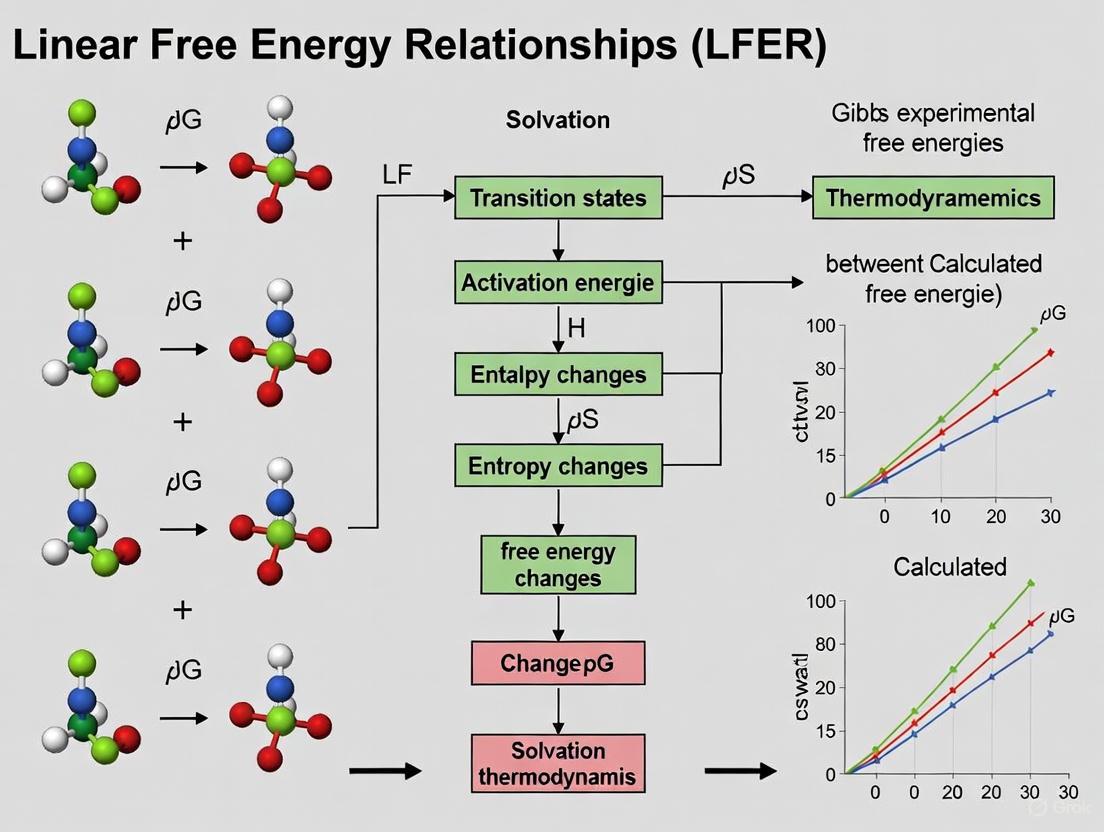
The concept of free energy is foundational to understanding molecular interactions, as it quantifies the energetic driving forces behind biochemical processes, molecular recognition, and supramolecular assembly. In thermodynamics, free energy is a state function that represents the maximum amount of work a thermodynamic system can perform at constant temperature and pressure, with its sign indicating whether a process is thermodynamically favorable or forbidden [7]. Since free energy contains potential energy, it is not absolute but depends on the choice of a zero point, making only relative free energy values or changes in free energy physically meaningful [7]. For researchers in solvation thermodynamics and drug development, connecting these macroscopic thermodynamic quantities to the microscopic world of molecular interactions provides critical insights for predicting binding affinity, protein folding, and solute partitioning behavior.
The Gibbs free energy (G), defined as G = H - TS (where H is enthalpy, T is absolute temperature, and S is entropy), is particularly useful for processes involving a system at constant pressure and temperature, as it subsumes entropy changes due to heat and excludes p dV work [7]. This makes it indispensable for solution-phase chemists and biochemists studying molecular interactions in biological systems. The historically earlier Helmholtz free energy (A = U - TS), where U is internal energy, is completely general and its decrease represents the maximum amount of work which can be done by a system at constant temperature [7].
Within the context of Linear Free Energy Relationships (LFERs) in solvation thermodynamics research, these fundamental concepts provide the theoretical foundation for understanding how molecular descriptors correlate with thermodynamic properties across different compounds. The Abraham solvation parameter model, known alternatively as the Linear Solvation Energy Relationships (LSER) model, has seen remarkable success in numerous applications across the chemical, biochemical, and environmental sectors [3]. Understanding the thermodynamic basis of LFER linearity is essential for the evaluation and exchange of thermodynamic quantities between models and databases [3].
Molecular Interactions and Their Energetic Signatures
Molecular recognition in biological systems depends on a complex balance of weak, cooperative interactions that enable the functional flexibility observed in biomolecules [8]. While covalent bonds (with energies typically 348-336 kJ/mol) provide structural integrity, the weaker non-covalent interactions (typically 4-29 kJ/mol) govern molecular recognition, protein folding, and self-assembly processes [8]. The cooperative nature of hydrogen bonding between complementary nitrogenous bases, for instance, maintains the double-stranded structure of DNA while allowing for separation during replication and transcription [8].
Table 1: Types of Molecular Interactions and Their Properties
| Interaction Type | Functional Form | Approximate Energy Range | Role in Molecular Systems |
|---|---|---|---|
| Covalent bonds | Complex, short-range | 336-348 kJ/mol | Molecular backbone structure |
| Charge-charge (ionic) | E ∝ 1/d | 40-80 kJ/mol (in vacuum) | Strong electrostatic attraction |
| Hydrogen bonding | E ∝ -1/d² (approx.) | 4-29 kJ/mol | Molecular recognition, specificity |
| Charge-dipole | E ∝ 1/d² (fixed) | 15-50 kJ/mol | Solvation, hydration shells |
| Dipole-dipole | E ∝ 1/d³ (fixed) | 2-10 kJ/mol | Intermolecular attraction |
| Van der Waals | E ∝ 1/d⁶ | 1-5 kJ/mol | Universal attraction |
| Hydrophobic effect | Entropy-driven | Varies with surface area | Protein folding, membrane formation |
The hydrophobic interaction represents a particularly important driving force in biological systems, where the transfer of nonpolar groups to aqueous phases results in a positive free energy change due to entropic decreases of surrounding water molecules [8]. For methane, with a molecular surface area of approximately 0.50 nm², the free energy of transfer to water is +14.5 kJ/mol, equivalent to 48 mJ/m² [8]. This effect is responsible for protein folding and the formation of supramolecular lipid aggregates such as biological membranes [8].
The intervening medium dramatically modulates electrostatic interactions through its dielectric constant. Water, with a dielectric constant of 78.5 at 25°C, effectively screens electrostatic interactions, while hydrocarbon environments like dodecane (ε = 2.0) act as insulators [8]. This dielectric screening is particularly important in protein-ligand binding, where the local environment can vary from highly polar to largely hydrophobic.
Linear Free Energy Relationships in Solvation Thermodynamics
Linear Free Energy Relationships (LFERs) provide powerful correlative frameworks that connect molecular structure to thermodynamic behavior across compound series. The Abraham solvation parameter model, alternatively known as the Linear Solvation Energy Relationships (LSER) model, has demonstrated remarkable success across chemical, biochemical, and environmental applications [3]. This model establishes linear relationships between free energy-based properties and molecular descriptors that encode different aspects of molecular interactions.
The thermodynamic basis for LFER linearity can be understood through a combination of equation-of-state solvation thermodynamics with the statistical thermodynamics of hydrogen bonding [3]. This theoretical foundation explains what the linearity entails and provides insights into how it can be interpreted and extended for predictions across broad ranges of external conditions. Recent advances have focused on predicting solvent LFER coefficients from corresponding molecular descriptors, which are known for thousands of compounds, significantly enhancing the model's predictive capacity in practical applications [3].
LFER approaches find particularly valuable applications in:
- Solvent screening for industrial and pharmaceutical processes
- Solute partitioning between different phases in extraction and chromatography
- Activity coefficients at infinite dilution for thermodynamic modeling
- Hydration and solvation energies for environmental fate prediction
- Drug binding affinity estimation in pharmaceutical development
The linear relationships observed in these systems emerge from the proportional contributions of different interaction types to the overall free energy change, with the coefficients in LFER equations representing the susceptibility of the process to specific molecular properties.
Experimental Protocols in Free Energy Calculations
Accurate free-energy calculations provide mechanistic insights into molecular recognition and conformational equilibrium, offering valuable tools for drug development professionals [9]. These computational methods enable researchers to study thermodynamic properties of different states of molecular systems in their equilibrium basin and obtain accurate absolute binding free-energy calculations for protein-ligand binding.
Mining Minima (M2) Methodology
The M2 algorithm represents an endpoint free energy method that approximates the overall free energy of a molecular system by identifying a manageable set of conformations (local energy minima) and summing the computed configuration integral of each energy minimum [9]. The standard binding free energy can be calculated as:
ΔG° = G°{PL} - G°{P} - G°_{L}
where G°{PL}, G°{P}, and G°{L} represent the standard free energies of the protein-ligand complex, free protein, and free ligand, respectively [9]. The standard free energy of each molecule (G°X) is calculated by summing contributions from N local energy wells:
G°X = -RT ln(∑{i=1}^N e^{-G°_i/RT})
where G°_i represents the standard free energy from distinct energy wells [9].
Table 2: Research Reagent Solutions for Free Energy Calculations
| Reagent/Resource | Function/Purpose | Application Context |
|---|---|---|
| VM2 Software Package | Implements M2 algorithm for free energy calculations | Conformational searching and free energy integration |
| Amber10 Package | Molecular dynamics force field and parameters | Energy minimization and molecular mechanics calculations |
| Protein Data Bank Structures | Experimental templates for computational modeling | Provides initial coordinates (e.g., PDB: 1a9u, 1w82) |
| Explicit Solvent Models | Water representation for solvation thermodynamics | Solvation free energy calculations |
| Hessian Matrix Calculations | Bond-angle-torsion coordinate analysis | Harmonic approximation with anharmonicity correction |
| Flexible Region Definitions | User-defined flexible protein residues (e.g., within 7Å of ligands) | Reduces computational cost while maintaining accuracy |
Application to Protein-Ligand Systems
In practice, free energy calculations have been successfully applied to study challenging biological systems such as p38α mitogen-activated protein kinase (MAPK), a serine-threonine kinase important for regulating proinflammatory cytokines and a drug target for inflammatory diseases [9]. These calculations provide insights into the DFG-in and DFG-out equilibrium of the conserved Asp-Phe-Gly motif, which is crucial for kinase activation and inhibitor binding.
The computational protocol typically involves:
- Structure preparation using crystal structures from the Protein Data Bank as templates
- Conformational sampling through multiple iterations until free energy convergence
- Flexibility management by defining rigid and flexible regions to reduce computational cost
- Free energy computation using the M2 algorithm with enhanced harmonic approximation
- Analysis of energetic components and configurational entropy contributions
For a typical ligand-protein complex, one iteration may take 12-14 hours using four cores of an Intel Xeon 2.4 GHz CPU, with multiple iterations required for convergence [9]. This approach reveals multiple stable complex conformations, changes in protein and inhibitor conformations, and the balance between various energetic terms and configurational entropy loss during binding [9].
Thermodynamic Basis of LFER Linearity
The remarkable linearity observed in Linear Free Energy Relationships finds its foundation in the fundamental principles of solvation thermodynamics. Recent research has elucidated how the combination of equation-of-state solvation thermodynamics with the statistical thermodynamics of hydrogen bonding provides a rigorous explanation for LFER linearity at the thermodynamic level [3]. This theoretical understanding is essential for proper evaluation and exchange of thermodynamic quantities between models and databases.
The linear relationships emerge because the free energy changes associated with solvation processes can be decomposed into contributions from different types of molecular interactions, each scaling linearly with appropriate molecular descriptors. For the Abraham LSER model, these descriptors typically encode information about:
- Hydrogen-bond donor and acceptor capabilities
- Molecular volume and polarizability
- Dipolarity/polarizability interactions
- Charge-transfer characteristics
The thermodynamic basis for this decomposition lies in the separability of interaction free energy contributions under certain conditions, where cross-terms remain relatively constant or scale proportionally across congeneric series of compounds. This theoretical framework not only explains existing LFER relationships but also enables extension of these models to predict behavior across broader ranges of external conditions, significantly enhancing their utility in practical applications like solvent screening and solute partitioning prediction [3].
Understanding this thermodynamic basis allows researchers to critically evaluate the limitations of LFER approaches and identify situations where nonlinear behavior might be expected, such as when significant conformational changes occur or when specific directional interactions dominate the binding process. For drug development professionals, this knowledge provides a foundation for interpreting LFER-based predictions of binding affinity and optimizing molecular structures to enhance specificity and potency.
The Linear Solvation Energy Relationship (LSER) model, pioneered by Abraham, stands as one of the most successful predictive frameworks in solvation thermodynamics. This technical guide deconstructs the fundamental LSER equation, examining the physical interpretation of its six core molecular descriptors and their thermodynamic significance within broader Linear Free-Energy Relationship (LFER) research. By exploring both traditional parameterization methods and emerging quantum-chemical approaches, we provide researchers with a comprehensive understanding of descriptor derivation, application, and current methodological evolution. The integration of computational chemistry with LSER principles promises enhanced predictive capability for solvation phenomena across chemical, pharmaceutical, and environmental disciplines.
The Linear Solvation Energy Relationship (LSER) model, developed by Abraham and colleagues, represents a cornerstone of modern solvation thermodynamics and Quantitative Structure-Property Relationship (QSPR) methodology [10] [2]. This robust predictive framework quantifies solute transfer between phases using linear free-energy relationships that correlate molecular descriptors with thermodynamic properties. The LSER approach has demonstrated remarkable success across diverse applications including solvent screening, partition coefficient prediction, and pharmaceutical design, often outperforming more computationally intensive models [10]. Its enduring utility stems from an elegant balance between molecular insight and practical predictive capability.
At its core, the LSER model provides a thermodynamic bridge between microscopic molecular interactions and macroscopic equilibrium properties. The model's theoretical foundation connects solvation free energies with practical phase equilibrium calculations through the fundamental relationship:
ΔG₁₂/RT = ln(φ₁⁰P₁⁰V_m₂γ₁₂^∞/RT) [10]
where ΔG₁₂ is the solvation free energy, γ₁₂^∞ is the activity coefficient at infinite dilution, P₁⁰ is the vapor pressure, V_m₂ is the molar volume of the solvent, and φ₁⁰ is the fugacity coefficient. This connection explains the significant interest in LSER models for thermodynamic calculations, particularly in chemical engineering applications where predicting phase behavior is crucial [10].
The LSER Equation: Mathematical Framework and Thermodynamic Basis
Fundamental LSER Equations
The LSER model employs simple linear equations to quantify solute transfer between phases. Two primary forms govern the most common applications:
For gas-to-liquid partitioning: Log KG = -ΔG₁₂/(2.303RT) = cg + egE + sgS + agA + bgB + l_gL [10]
For solvation enthalpy: Log KE = -ΔH₁₂/(2.303RT) = ce + eeE + seS + aeA + beB + l_eL [10]
Analogous equations describe solute transfer between two condensed phases [2]. In these equations, uppercase letters (E, S, A, B, V_x, L) represent solute-specific molecular descriptors, while lowercase coefficients (e, s, a, b, v, l) are solvent-specific system parameters that quantify the complementary effect of the solvent on solute-solvent interactions [2]. These system-specific coefficients are typically determined through multilinear regression of experimental data [2].
Thermodynamic Foundation
The theoretical basis for LSER's linearity, even for strong specific interactions like hydrogen bonding, stems from its foundation in solution thermodynamics [2]. When combined with the statistical thermodynamics of hydrogen bonding, the equation-of-state solvation thermodynamics provides a verifiable basis for the observed linear relationships in LSER equations [2]. This thermodynamic grounding enables the model to extract meaningful information about intermolecular interactions that can be transferred to other LFER-type models, acidity/basicity scales, or equation-of-state models [10].
Table 1: Components of the Fundamental LSER Equation for Gas-to-Liquid Partitioning
| Symbol | Term Type | Physical Interpretation |
|---|---|---|
| K_G | Variable | Gas-to-liquid partition coefficient |
| ΔG₁₂ | Variable | Solvation free energy |
| c_g | Constant | System-specific intercept |
| eg, sg, ag, bg, l_g | Coefficients | Solvent-specific interaction parameters |
| E, S, A, B, L | Descriptors | Solute-specific molecular descriptors |
Molecular Descriptors: Physical Meaning and Interpretation
Comprehensive Descriptor Definitions
The LSER model characterizes solutes through six fundamental molecular descriptors that collectively capture the dominant intermolecular interaction types:
V_x - McGowan's Characteristic Volume: Represents the molecular volume calculated from atomic volumes and bond contributions, corresponding to the cavity formation energy required to accommodate the solute in the solvent [2]. This descriptor primarily reflects dispersive interactions with solvent molecules and is mathematically related to the molecular size [11].
L - Gas-Hexadecane Partition Coefficient: Defined as the equilibrium constant for gas-liquid partition in n-hexadecane at 298 K, this descriptor characterizes dispersion interactions with an inert alkane reference solvent [10] [2]. It serves as a measure of the solute's ability to participate in London dispersion forces.
E - Excess Molar Refraction: Derived from the solute's refractive index, this descriptor quantifies the solute's ability to engage in polarization interactions, particularly those involving π- and n-electrons [10] [2]. It represents the contribution of electron-rich regions to overall solvation energy.
S - Dipolarity/Polarizability: Captures the solute's overall polarity and ability to stabilize charge separation, encompassing both permanent dipole-permanent dipole (Keesom) and dipole-induced dipole (Debye) interactions [10] [2]. This descriptor reflects the molecule's response to electrostatic fields.
A - Hydrogen Bond Acidity: Quantifies the solute's capacity to donate hydrogen bonds (proton donor strength) [10] [2]. This descriptor is particularly important in pharmaceutical applications where specific hydrogen bonding interactions often determine biological activity.
B - Hydrogen Bond Basicity: Measures the solute's capacity to accept hydrogen bonds (proton acceptor strength) [10] [2]. Like its acidic counterpart, this descriptor plays a crucial role in determining solvation behavior in protic environments.
Table 2: LSER Molecular Descriptors and Their Physical Significance
| Descriptor | Interaction Type | Molecular Property | Determination Method |
|---|---|---|---|
| V_x | Dispersion | Molecular volume | Atomic contribution calculations |
| L | Dispersion | Gas-hexadecane partitioning | Experimental measurement |
| E | Polarization | Electron-rich character | Refractive index derivation |
| S | Dipolarity | Overall molecular polarity | Solvatochromic comparison |
| A | Hydrogen bonding | Proton donor capacity | Thermodynamic/spectroscopic measurement |
| B | Hydrogen bonding | Proton acceptor capacity | Thermodynamic/spectroscopic measurement |
Thermodynamic Interpretation of Descriptor Contributions
In the LSER framework, the products of solute descriptors and solvent coefficients directly correlate with contributions to the overall free energy of solvation. Specifically, the terms aA and bB represent the hydrogen bonding contribution to solvation free energy, while the corresponding terms in the enthalpy equation quantify the hydrogen bonding contribution to solvation enthalpy [2]. This separation of interaction types enables researchers to deconstruct complex solvation phenomena into physically meaningful components, facilitating rational solvent selection and molecular design.
Methodological Approaches for Descriptor Determination
Experimental Parameterization Methods
Traditional LSER parameterization relies heavily on experimental data from various sources:
Multilinear Regression: The primary method for determining both molecular descriptors and system-specific coefficients involves multilinear regression of extensive experimental partition coefficient and solvation data [10] [2]. This approach requires high-quality, critically evaluated datasets for numerous solute-solvent combinations.
Chromatographic Measurements: Retention data from gas-liquid chromatography provides experimental partition coefficients for numerous compounds, enabling descriptor determination through systematic column characterization [11].
Solvatochromic Studies: UV-Vis spectroscopy of indicator dyes in different solvents establishes polarity scales that correlate with LSER descriptors, particularly for polarizability and hydrogen bonding parameters [11].
Calorimetric Methods: Measurement of enthalpies of solvation or hydrogen bond formation provides direct thermodynamic data for parameterizing the enthalpy-based LSER equations [11].
The experimental approach, while historically valuable, faces significant limitations. Model expansion becomes constrained by experimental data availability, and issues of thermodynamic inconsistency arise, particularly in self-solvation of hydrogen-bonded compounds where solute and solvent become identical [10].
Quantum-Chemical Determination of Descriptors
Recent advances address traditional limitations through quantum-chemical (QC) approaches:
COSMO-Based Descriptors: New QC-LSER methodologies derive molecular descriptors from molecular surface charge distributions obtained from COSMO-type quantum chemical calculations [10]. These descriptors provide a thermodynamically consistent framework for LSER parameterization.
Sigma Profile Analysis: The distribution of screening charges on the molecular surface (sigma profiles) enables calculation of hydrogen bonding capacities directly from molecular structure [12]. This approach facilitates descriptor prediction for compounds without experimental data.
Direct DFT Calculations: Density functional theory calculations provide a priori prediction of molecular descriptors, particularly for hydrogen bonding parameters (α and β) that correlate with traditional A and B descriptors [12]. The relationship takes the form: ΔE_HB = 2.303RT(α₁β₂ + α₂β₁) for hydrogen-bonding interaction energy.
Figure 1: Quantum-Chemical Workflow for LSER Descriptor Determination
Successful LSER research requires specialized tools and resources spanning computational and experimental domains:
Table 3: Essential Research Resources for LSER Studies
| Resource Category | Specific Tools/Methods | Primary Application | Key Function |
|---|---|---|---|
| Computational Chemistry | COSMO-RS (COSMOtherm) | Sigma profile generation | Molecular charge distribution calculation |
| Quantum Chemistry Software | DFT suites (Gaussian, ORCA) | Electronic structure calculation | Wavefunction optimization for descriptor prediction |
| LSER Databases | Abraham LSER Database | Descriptor retrieval | Experimental parameter repository |
| Statistical Analysis | Multilinear regression algorithms | Model parameterization | Coefficient and descriptor optimization |
| Experimental Characterization | Gas-liquid chromatography | Partition coefficient measurement | Experimental L descriptor determination |
| Solvatochromic Probes | UV-Vis spectroscopy with indicator dyes | Polarity assessment | S descriptor estimation |
Current Developments and Future Perspectives
Integration with Equation-of-State Thermodynamics
Recent research focuses on bridging LSER with equation-of-state models through Partial Solvation Parameters (PSP) [2]. This integration aims to extract thermodynamic information from the LSER database for use in predictive thermodynamic models over extended temperature and pressure ranges. The PSP approach defines parameters (σd, σp, σa, σb) corresponding to dispersion, polar, acidic, and basic interactions that demonstrate one-to-one correspondence with LSER molecular descriptors [11]. This interconnection facilitates information exchange between QSPR-type databases and equation-of-state developments.
Quantum-Chemical LSER (QC-LSER) Advancements
The integration of quantum chemistry with LSER principles represents the cutting edge of methodology development:
Thermodynamically Consistent Reformulation: New QC-LSER approaches enable thermodynamically consistent reformulation of LSER models, permitting extraction of valuable information on intermolecular interactions and its transfer to other model frameworks [10].
Hydrogen-Bonding Quantification: QC-LSER methods now provide improved prediction of hydrogen-bonding free energies, enthalpies, and entropies for diverse solutes, addressing previous inconsistencies in self-solvation calculations [10] [12].
Conformational Analysis: Emerging methods address the role of conformational changes in solvation quantities, leveraging quantum chemical calculations to account for population distributions in multi-conformer systems [12].
Figure 2: LSER Methodology Integration and Future Directions
The deconstruction of the LSER equation reveals a sophisticated yet practical framework for understanding and predicting solvation phenomena. The six molecular descriptors—V_x, L, E, S, A, and B—provide a physically meaningful representation of key intermolecular interactions that govern solute partitioning between phases. While traditional experimental approaches remain valuable, the integration of quantum chemical methodologies addresses previous limitations and enhances predictive capability. The ongoing integration of LSER with equation-of-state models through Partial Solvation Parameters and COSMO-based descriptors represents a promising direction for expanding the model's applicability across chemical engineering, pharmaceutical development, and environmental science. As methodology continues to evolve, the fundamental LSER equation maintains its position as an essential tool for researchers seeking to connect molecular structure with thermodynamic behavior.
The Statistical Thermodynamics Underpinning LFER Linearity
Linear Free Energy Relationships (LFERs) are foundational tools in physical organic chemistry, environmental science, and pharmaceutical research for predicting how molecular structure influences chemical reactivity and partitioning behavior. While their empirical success is well-documented, the fundamental thermodynamic principles governing their linearity have remained less explored. This whitepaper examines the statistical thermodynamic basis of LFER linearity, focusing specifically on solvation processes within the context of the Abraham solvation parameter model, also known as the Linear Solvation Energy Relationships (LSER) model. Understanding this thermodynamic foundation is crucial for researchers leveraging LFERs in drug development, where accurate prediction of solvation, partitioning, and binding interactions directly impacts compound optimization and efficacy.
The remarkable linearity observed in LFERs, even for strong specific interactions like hydrogen bonding, presents a theoretical puzzle that conventional explanations struggle to fully address. Recent advances combining equation-of-state solvation thermodynamics with the statistical thermodynamics of hydrogen bonding now provide a coherent framework explaining this behavior [2]. This whitepaper synthesizes these advances to illuminate the thermodynamic machinery underlying LFER linearity, enabling more informed application and extension of these valuable relationships in research settings.
Theoretical Framework
LFER Formalism and Molecular Descriptors
The Abraham LFER model quantifies solute transfer between phases through two primary relationships. For transfer between condensed phases:
[\text{log}(P) = cp + epE + spS + apA + bpB + vpV_x] [2]
And for gas-to-solvent partitioning:
[\text{log}(KS) = ck + ekE + skS + akA + bkB + l_kL] [2]
In these equations, the uppercase letters represent solute-specific molecular descriptors:
- E: Excess molar refraction
- S: Polarity/polarizability
- A: Hydrogen bond acidity
- B: Hydrogen bond basicity
- V_x: McGowan's characteristic volume
- L: Gas-hexadecane partition coefficient [2] [13]
The lowercase coefficients ((ep), (sp), (a_p), etc.) are system-specific parameters reflecting the complementary properties of the solvent or phase. These are typically determined through multivariate linear regression against experimental data [2].
Thermodynamic Foundation of Linearity
The linearity of free-energy-based properties in LFERs arises from fundamental thermodynamic compensation effects. For processes in solution, there exists a general tendency for enthalpies ((ΔH)) and entropies ((ΔS)) to compensate each other such that changes in free energy ((ΔG = ΔH - TΔS)) are much smaller and exhibit simpler relationships than the individual components [14].
This compensation is particularly pronounced for solvent-solute interactions. Any interaction that strengthens binding between solute and solvent molecules typically lowers the enthalpy ((ΔH) becomes more negative) but simultaneously restricts the freedom of vibration and rotation of solvent molecules, lowering the entropy ((-TΔS) becomes more positive). The result is partial compensation that yields a much smaller effect on the free energy ((ΔG)) [14].
When this compensation is approximately linear across a series of related compounds or conditions, it produces the linear free energy relationships observed in LFERs. The mathematical expression of this phenomenon can be represented as:
[TΔS = αΔH + β]
where (α) and (β) are constants for a given series. Substituting into the Gibbs free energy equation:
[ΔG = ΔH - TΔS = ΔH - (αΔH + β) = (1-α)ΔH - β]
This relationship demonstrates that when (α ≈ 1), (ΔG) becomes largely independent of (ΔH), explaining why free energies often show simpler, more linear relationships than the corresponding enthalpy changes [14].
Table 1: Key Molecular Descriptors in Abraham LFER Model
| Descriptor | Symbol | Molecular Property Represented | Typical Range |
|---|---|---|---|
| Excess Molar Refraction | E | Polarizability from π- and n-electrons | -0.1 to 3.63 |
| Dipolarity/Polarizability | S | Polarity and polarizability | 0 to 1.98 |
| Hydrogen Bond Acidity | A | Hydrogen bond donating ability | 0 to 0.69 |
| Hydrogen Bond Basicity | B | Hydrogen bond accepting capacity | 0 to 1.28 |
| McGowan Characteristic Volume | V_x | Molecular size | 0.79 to 1.44 |
| Hexadecane-Air Partition Coefficient | L | Dispersion interactions | 3 to 11.74 |
Statistical Thermodynamics of Hydrogen Bonding
The treatment of hydrogen bonding interactions presents a particular challenge in understanding LFER linearity, as these strong, specific interactions might be expected to exhibit more complex behavior. The resolution lies in the statistical thermodynamics of hydrogen bonding in solution.
When a hydrogen bond forms between solute and solvent, there is a free energy change ((ΔG{hb})) that can be partitioned into enthalpy ((ΔH{hb})) and entropy ((ΔS_{hb})) components. The key insight is that even for these specific interactions, the relationship between the probability of bond formation and the free energy change follows a statistical thermodynamic model that maintains linearity in free energy relationships [2].
The hydrogen bonding contribution to solvation free energy can be expressed through a Boltzmann factor:
[P{hb} \propto \exp\left(-\frac{ΔG{hb}}{RT}\right)]
where (P_{hb}) represents the probability of hydrogen bond formation. In the LFER formalism, this translates to linear contributions from the A (acidity) and B (basicity) descriptors through their products with the corresponding system coefficients a and b [2].
For a solute with hydrogen bond acidity A₁ in a solvent with basicity coefficient b₂, the contribution to log(P) is approximately linear in A₁·b₂, and similarly for basic solutes in acidic solvents. This linearity persists because the probability of hydrogen bond formation depends exponentially on the free energy change, but for small changes relative to RT, the relationship between molecular descriptors and log(P) remains approximately linear [2].
Partial Solvation Parameters (PSP) Framework
The Partial Solvation Parameters (PSP) framework provides a bridge between the empirical LFER descriptors and fundamental equation-of-state thermodynamics. This approach defines four key parameters that collectively describe a molecule's solvation behavior:
- σ_d: Dispersion PSP, reflecting weak dispersive interactions
- σ_p: Polar PSP, collectively reflecting Keesom-type and Debye-type polar interactions
- σ_a: Hydrogen-bonding acidity PSP
- σ_b: Hydrogen-bonding basicity PSP [2]
These PSPs have an equation-of-state basis that allows estimation over a broad range of external conditions, unlike the original LFER parameters which are typically defined at standard conditions. The hydrogen-bonding PSPs (σa and σb) are particularly important as they enable estimation of the free energy change upon hydrogen bond formation ((ΔG{hb})), along with the corresponding enthalpy ((ΔH{hb})) and entropy ((ΔS_{hb})) changes [2].
Table 2: Experimental Ranges for Partition Coefficients in Protein-Water Systems
| System | Partition Coefficient | Range (log units) | Number of Data Points | Key Applications |
|---|---|---|---|---|
| Structural Protein-Water | log K_pw | 0.6 to 4.9 | 46 (chicken) + 45 (fish) | Chemical fate, food web accumulation |
| Bovine Serum Albumin-Water | log K_BSA | 1.5 to 4.8 | 83 | Pharmacokinetics, serum binding |
| Octanol-Water | log K_ow | 1.4 to 6.8 | Varies | Standard hydrophobicity measure |
| Air-Water | log K_aw | -10.6 to 2.2 | Varies | Volatility assessment |
LFERs in Biological Partitioning
The thermodynamic principles underlying LFER linearity find important application in predicting biological partitioning behavior, particularly relevant to drug development. Recent advances have demonstrated the effectiveness of simplified two-parameter LFER (2p-LFER) models for predicting protein-water partition coefficients [13].
These models leverage the finding that the six-dimensional intermolecular interaction space defined by Abraham descriptors can be efficiently simplified to two key dimensions represented by octanol-water (log Kow) and air-water (log Kaw) partition coefficients. The 2p-LFER model takes the form:
[\text{log } K{pw} = α\cdot\text{log } K{ow} + β\cdot\text{log } K_{aw} + γ]
where α, β, and γ are fitted parameters [13].
This model achieves impressive predictive accuracy for structural protein-water partition coefficients (R² = 0.878, RMSE = 0.334) and bovine serum albumin-water partition coefficients (R² = 0.760, RMSE = 0.422), performance comparable to the more parameter-intensive polyparameter LFER approach [13].
The success of these simplified models further supports the thermodynamic basis of LFER linearity, demonstrating that the complex interplay of intermolecular interactions can be captured through linear combinations of macroscopic properties like hydrophobicity (log Kow) and volatility (log Kaw).
Experimental Protocols and Methodologies
Determining LFER System Coefficients
The determination of system-specific coefficients in LFER equations follows well-established protocols:
Data Collection: Compile experimental partition coefficient data (log P or log K) for a diverse set of solutes with known Abraham descriptors in the system of interest. The training set should encompass a wide range of E, S, A, B, and V values to ensure model robustness [13].
Multiple Linear Regression: Perform multivariate linear regression using the equation: [ \text{log}(P) = cp + epE + spS + apA + bpB + vpV_x] where the lowercase coefficients are determined through least-squares fitting [2] [13].
Validation: Verify model performance using leave-one-out cross-validation or an independent test set. The model should explain at least 85-90% of variance (R² > 0.85) with residuals randomly distributed [13].
Application: Use the fitted equation to predict partition coefficients for new compounds with known Abraham descriptors within the defined chemical space [13].
Hydrogen Bonding Contribution Quantification
To experimentally isolate hydrogen bonding contributions to solvation free energy:
Isosteric Compound Design: Design molecular pairs where one molecule contains a hydrogen bond donor/acceptor and its isosteric counterpart lacks this functionality while maintaining similar size and polarizability [2].
Partition Coefficient Measurement: Measure partition coefficients for both compounds in the system of interest using appropriate analytical methods (e.g., HPLC, shake-flask) [13].
Difference Analysis: The difference in log P values between the hydrogen-bonding and non-hydrogen-bonding analogs provides an experimental measure of the hydrogen bonding contribution [2].
Thermodynamic Profiling: For complete characterization, measure temperature dependence to extract enthalpic and entropic contributions to hydrogen bonding [2].
Experimental Workflow for Hydrogen Bonding Contribution Analysis
Research Reagent Solutions
Table 3: Essential Research Reagents for LFER Thermodynamics Studies
| Reagent/Material | Function/Application | Technical Specifications | Thermodynamic Relevance |
|---|---|---|---|
| n-Hexadecane | Reference solvent for dispersion interactions | High purity (>99%), measures L descriptor [13] | Isolates weak dispersive forces from specific interactions |
| Water (HPLC Grade) | Reference polar solvent | Low organic content, measures A/B descriptors [13] | Provides baseline for hydrogen bonding and polar interactions |
| Octanol (n-Octanol) | Standard partitioning solvent | >99% purity, pre-saturated with water [13] | Reference system for hydrophobicity (log K_ow) |
| Buffer Solutions (Various pH) | Control ionization state | Specific pH ±0.01 units, constant ionic strength | Isolates neutral species partitioning for LFER development |
| Deuterated Solvents | NMR spectroscopy for binding studies | 99.8% D minimum, water content <0.01% | Quantifies binding constants and stoichiometry |
| SPME Fibers | Headspace analysis for K_aw | Various coatings (PDMS, CAR/PDMS) | Measures gas-phase partitioning for volatility assessment |
| HPLC Columns (C18, HILIC) | Partition coefficient measurement | Specific particle size (e.g., 5μm), defined surface chemistry | High-throughput log P/K measurement for LFER development |
The statistical thermodynamics underpinning LFER linearity reveals a sophisticated compensation mechanism between enthalpy and entropy changes in solvation processes. This framework explains why free energy relationships remain linear even for strong specific interactions like hydrogen bonding, where complex behavior might otherwise be expected. The combination of equation-of-state solvation thermodynamics with the statistical thermodynamics of hydrogen bonding provides a fundamental basis for the empirical success of LFER approaches in chemical and pharmaceutical research.
For drug development professionals, this thermodynamic understanding enables more informed application of LFER predictions to bioavailability, membrane permeability, and protein binding assessments. The continued development of Partial Solvation Parameters and related frameworks promises enhanced predictive capability across wider ranges of conditions, supporting more efficient drug design and optimization workflows.
Thermodynamic Basis of LFER Linearity
Bridging Solvation Thermodynamics and Classical Phase Equilibria
This technical guide explores the fundamental integration of solvation thermodynamics with classical phase equilibrium principles, framed within the context of Linear Free-Energy Relationships (LFER) in solvation research. The solvation free energy (ΔG°), a cornerstone quantity in molecular thermodynamics, provides a critical bridge between microscopic solute-solvent interactions and macroscopic phase behavior. By examining the thermodynamic foundations of LFER models and their application across chemical, biochemical, and environmental domains, this work establishes how solvation parameters enable predictive modeling of solute transfer and partitioning between phases. The explicit mathematical relationships connecting solvation constants with activity coefficients, vapor pressures, and partition coefficients demonstrate how molecular-scale interactions dictate macroscopic phase distribution. Through detailed methodologies, data presentation, and visualization tools, this guide provides researchers and drug development professionals with a comprehensive framework for leveraging LFER principles in practical applications ranging from solvent screening to biomolecular stabilization.
Solvation thermodynamics provides the fundamental link between molecular-level interactions and macroscopic phase behavior that governs countless chemical and biological processes. The free energy change upon solvation of a solute in a solvent (ΔG°), along with its enthalpic (ΔH°) and entropic (ΔS°) components, serves as the critical connection point between these domains. As established by Panayiotou et al., these solvation quantities "play an important role in molecular thermodynamics and computational chemistry, since they can make a significant contribution to the total free energy of chemical reactions in solution" [15].
The Abraham solvation parameter model, alternatively known as the Linear Solvation Energy Relationship (LSER) model, represents one of the most successful frameworks for quantifying and predicting these relationships [3]. Its remarkable success across chemical, biochemical, and environmental applications stems from its ability to correlate extensive experimental solvation data through molecular descriptors that reflect interaction capacities between solutes and solvents. Understanding the thermodynamic basis of LFER linearity is essential for proper evaluation and exchange of thermodynamic quantities between models and databases [3].
For drug development professionals, these relationships prove particularly valuable in predicting partition coefficients, solubility, and permeability – key factors determining drug absorption, distribution, and efficacy. The connection between solvation thermodynamics and classical phase equilibria enables rational design of physicochemical processes, stabilization of biomolecules, controlled drug delivery systems, and metabolic pathway analysis [15].
Theoretical Foundations
Fundamental Thermodynamic Relationships
The mathematical bridge between solvation thermodynamics and classical phase equilibria is established through several key equations that connect molecular interactions with measurable macroscopic properties. For the solvation of solute 1 in solvent 2, the fundamental relationship is expressed as [15]:
Where K₁₂° is the equilibrium solvation constant, ΔG₁₂° is the solvation free energy, ΔH₁₂° is the solvation enthalpy, ΔS₁₂° is the solvation entropy, φ₁° is the fugacity coefficient of the pure solute, P₁° is the vapor pressure of the pure solute, V_m₂ is the molar volume of the solvent, and γ₁₂^∞ is the activity coefficient of the solute at infinite dilution in the solvent.
For pure solvents at ambient conditions, this relationship simplifies to the self-solvation free energy expression [15]:
The self-solvation enthalpy (-ΔH°) becomes equivalent to the heat of vaporization (ΔH_vap), leading to the self-solvation entropy expression [15]:
These equations establish the direct connection between solvation thermodynamics and classical thermodynamic properties of pure substances, enabling the calculation of solvation parameters from readily available physical property data.
Linear Solvation Energy Relationships (LSER)
The LSER model provides a quantitative framework for predicting solvation free energies through linear relationships incorporating molecular descriptors. The standard Abraham LSER model for solvation from the gas phase to a liquid solvent is expressed as [15]:
An alternative formulation for solute transfer between two condensed phases uses [15]:
Table 1: LSER Molecular Descriptors and Their Physical Significance
| Descriptor | Physical Significance | Application |
|---|---|---|
| V | McGowan's characteristic volume | Size-related interactions |
| L | Gas-liquid partition coefficient in n-hexadecane at 298K | Dispersion interactions |
| E | Excess molar refraction | Polarizability contributions |
| S | Polarity/polarizability | Dipole-dipole and induced dipole interactions |
| A | Hydrogen-bonding acidity | Proton donor capability |
| B | Hydrogen-bonding basicity | Proton acceptor capability |
The uppercase letters represent solute molecular descriptors, while the lowercase coefficients are solvent-specific parameters determined through multilinear regression of experimental data. This approach has been successfully applied to approximately 80 different solvents [15].
Thermodynamic Basis of LFER Linearity
The linearity of LFER relationships finds its foundation in the fundamental principles of solution thermodynamics. As explained by Panayiotou et al., "the equation-of-state solvation thermodynamics with the statistical thermodynamics of hydrogen bonding" provides the theoretical underpinning for this linearity [3]. This combination explains how the free energy of solvation can be decomposed into additive contributions from different interaction types, each proportional to specific molecular properties.
The division of intermolecular interactions into clear categories – electrostatic (polar) and non-electrostatic (non-polar, including dispersion) – provides the physical basis for this additive approach [15]. While real intermolecular interactions exist on a continuum without sharp boundaries, this division has proven remarkably effective for correlating and predicting solvation behavior across diverse chemical systems.
Computational Methodologies and Molecular Descriptors
Quantum Chemical Approaches to Molecular Descriptors
Recent advances have enabled the development of new molecular descriptors derived from quantum chemical calculations, particularly COSMO-type solvation models. These approaches provide a thermodynamically consistent reformulation of QSPR-type Linear Free-Energy Relationship models [16]. The new method utilizes "COSMO-type quantum chemical solvation calculations for the development of four new molecular descriptors of solutes for their electrostatic interactions" [15].
This approach significantly reduces the parameter requirements compared to traditional LSER models. Where the Abraham LSER model requires six solvent-specific parameters, the new model "needs one to three solvent-specific parameters for the prediction of solvation free energies" [15]. This reduction in parameterization demands while maintaining predictive capability represents a substantial advancement in computational efficiency.
The methodology involves:
- Quantum chemical calculations of molecular surface charge distributions (σ-profiles)
- Extraction of electrostatic interaction information from the resulting charge distributions
- Development of specific descriptors for dispersion, polar, and hydrogen-bonding contributions
- Parameterization against reference solvation free energy data, typically from Abraham's LSER database
New Model for Solvation Free Energy Contributions
A recently developed method enables the estimation of separate contributions to solvation free energy from dispersion, polar, and hydrogen-bonding intermolecular interactions [15]. This approach provides greater physical insight into the relative importance of different interaction types and facilitates information exchange with other quantitative structure-property relationship (QSPR) models.
The model employs "the very same molecular descriptors for the calculation of solvation enthalpies" [15], ensuring consistency across different thermodynamic properties. This unified treatment represents a significant advantage over traditional LSER approaches, where "all coefficients of Equation (4) are, in general, different (and, often, very different) from the corresponding coefficients of Equation (5)" [15], referring to the equations for solvation free energy and enthalpy, respectively.
Table 2: Comparison of Traditional and Emerging Solvation Modeling Approaches
| Aspect | Abraham LSER Model | New QC-Based Model |
|---|---|---|
| Parameters per solvent | 6 LFER coefficients | 1-3 solvent-specific parameters |
| Molecular descriptors | Experimentally derived E, S, A, B, V, L | Quantum chemically derived descriptors |
| Physical basis | Empirical correlation | Quantum chemical calculations with empirical parameterization |
| Consistency between ΔG° and ΔH° | Separate parameter sets | Unified descriptors for both properties |
| Hydrogen-bonding treatment | Incorporated in A and B descriptors | Explicit calculation with new descriptors |
Workflow for Solvation Free Energy Calculation
The following diagram illustrates the integrated workflow for calculating solvation free energies using both traditional LSER and modern quantum chemical approaches:
Experimental Protocols and Data Management
Data Management for FAIR Compliance
Proper data management practices are essential for ensuring the reproducibility and utility of solvation thermodynamics research. The FAIR Data principles (Findable, Accessible, Interoperable, Reusable) provide a framework for effective data stewardship [17]. Implementing these principles from the beginning of the data lifecycle, rather than attempting retroactive compliance, significantly reduces effort and improves data quality.
The ODAM (Open Data for Access and Mining) approach exemplifies this proactive methodology by focusing on "structural metadata related to the experimental data in the spreadsheets, i.e., how they are organized so that we can more easily exploit them" [17]. This strategy acknowledges that "researchers have the best control and understanding of their data, they are in the best position to annotate it" [17], while providing them with protocols and methods adapted to their IT skills.
Key steps in the data preparation protocol include [17]:
- Structured data collection using researcher-friendly tools (e.g., spreadsheets)
- Comprehensive annotation with links to accessible definitions and community-approved ontologies
- Description of structural metadata (e.g., links between data tables)
- Unambiguous definition of all internal elements (e.g., column definitions)
- Conversion to standard formats (e.g., Frictionless datapackage) for dissemination
LSER Parameter Determination Protocol
The experimental determination of LSER parameters follows a standardized protocol to ensure consistency and reliability:
Data Collection: Compile critically assessed experimental solvation data for diverse solutes in the target solvent. The database should include compounds representing the full range of possible molecular interactions.
Descriptor Assignment: Assign Abraham solute descriptors (E, S, A, B, V, L) to each compound based on experimental measurements or reliable prediction methods.
Multilinear Regression: Perform regression analysis according to the equation:
to determine the solvent-specific coefficients (c₂, e₂, s₂, a₂, b₂, l₂).
Validation: Verify the obtained parameters by predicting solvation free energies for compounds not included in the regression set and comparing with experimental values.
Documentation: Thoroughly document the data sources, regression statistics, and validation results to enable proper evaluation and reuse of the parameters.
This protocol has been successfully applied to determine LSER parameters for approximately 80 solvents, creating an extensive database for solvation thermodynamics applications [15].
Applications in Phase Equilibria Prediction
Predicting Partition Coefficients
A primary application of solvation thermodynamics lies in predicting solute partitioning between immiscible liquid phases. The partition coefficient of solute 1 between solvents 2 and 3 is obtained directly from the ratio of the equilibrium solvation constants [15]:
This relationship provides the fundamental connection between solvation free energies and partition coefficients, enabling prediction of solute distribution in extraction processes, drug delivery systems, and environmental partitioning.
The LSER model has been extensively applied to predict partition coefficients in diverse systems, including [15]:
- Water-organic solvent systems for liquid-liquid extraction
- Biological membrane partitioning for drug absorption prediction
- Environmental distribution between air, water, and soil phases
- Chromatographic retention in various stationary and mobile phase combinations
Activity Coefficients at Infinite Dilution
Solvation thermodynamics provides the foundation for predicting activity coefficients at infinite dilution (γ^∞), crucial for separation process design and solubility prediction. Equation (1) establishes the direct relationship between solvation free energy and activity coefficients:
This enables the calculation of γ^∞ from solvation free energies, or conversely, the determination of solvation parameters from experimentally measured activity coefficients. The LSER model has been particularly successful in correlating and predicting activity coefficients for system design in chemical engineering applications.
Bridging Atomistic and Continuum Scales
Recent work on phase equilibria in Ni-H systems demonstrates how solvation thermodynamics bridges atomistic simulations with continuum-scale modeling [18]. This approach "considers configurational entropy, an attractive hydrogen–hydrogen interaction, mechanical deformations and interfacial effects" to achieve "fully quantitative agreement in the chemical potential, without the need for any additional adjustable parameter" [18].
The free energy formulation for this scale-bridging approach includes multiple contributions [18]:
Where μ₀ is the solvation energy for an isolated hydrogen atom, NH is the number of hydrogen atoms, Fc is the configurational free energy, FH-H accounts for H-H interactions, and Fel represents elastic contributions. This comprehensive framework successfully captures phase coexistence behavior in metal-hydrogen systems, demonstrating the power of integrated thermodynamic modeling across scales.
Table 3: Essential Research Resources for Solvation Thermodynamics Studies
| Resource Category | Specific Examples | Function and Application |
|---|---|---|
| Computational Tools | COSMO-type quantum chemical solvation calculators | Generation of σ-profiles and electrostatic molecular descriptors |
| LSER parameter databases | Source of solvent-specific coefficients for solvation free energy predictions | |
| Statistical analysis software | Multilinear regression for LSER parameter determination | |
| Experimental Data Sources | Critically evaluated solvation databases | Source of experimental solvation free energies for parameterization |
| Vapor pressure and activity coefficient databases | Experimental data for solvation quantity calculations | |
| Heat of vaporization measurements | Determination of self-solvation enthalpies | |
| Molecular Descriptors | Abraham solute parameters (E, S, A, B, V, L) | Characterization of solute interaction capabilities |
| Quantum chemically derived descriptors | Alternative descriptors from molecular surface charge distributions | |
| Reference Systems | n-Hexadecane partition system | Reference for dispersion interaction characterization (L descriptor) |
| Specific hydrogen-bonding probes | Characterization of A (acidity) and B (basicity) descriptors |
The integration of solvation thermodynamics with classical phase equilibria through LFER principles provides a powerful framework for predicting and understanding molecular distribution across phases. The mathematical bridges established between solvation free energies and classical thermodynamic properties enable researchers to connect microscopic interactions with macroscopic behavior.
Future developments in this field are likely to focus on several key areas:
- Enhanced Molecular Descriptors: Continued refinement of quantum chemically derived descriptors will improve predictive accuracy while reducing parameterization requirements.
- Extended Temperature and Pressure Ranges: Developing models valid across broader ranges of external conditions will expand application domains.
- Machine Learning Integration: Combining LFER approaches with machine learning algorithms may capture non-linear relationships while maintaining physical interpretability.
- Complex System Applications: Extending these principles to increasingly complex systems, including ionic liquids, deep eutectic solvents, and biological environments.
The "complementary character" [15] of traditional LSER and emerging quantum chemical approaches suggests that hybrid methodologies will provide the most powerful solutions for future challenges in solvation thermodynamics and phase equilibria prediction. As these methods continue to evolve, they will further enhance our ability to design optimized processes and products across chemical, pharmaceutical, and environmental domains.
LSER Methodologies and Pharmaceutical Applications: From Theory to Practice
The Abraham Linear Solvation Energy Relationship (LSER) model is a cornerstone of solvation thermodynamics, providing a robust quantitative framework for predicting solute transfer between phases. As a specific implementation of Linear Free Energy Relationships (LFER), the model correlates a solute's partitioning behavior with its fundamental molecular properties, offering profound insights into the nature of intermolecular interactions that govern solubility, chromatographic retention, and other crucial physicochemical processes in chemical and pharmaceutical research [2]. The model's success stems from its ability to decompose complex solvation phenomena into discrete, physically meaningful interaction terms that collectively describe the free energy changes accompanying solute transfer.
The theoretical foundation of the Abraham model rests upon linear free energy relationships, which establish that the logarithm of a partition coefficient varies linearly with molecular descriptors characterizing solute-solvent interactions [19]. This linearity persists even for strong specific interactions like hydrogen bonding, finding its thermodynamic justification in the combination of equation-of-state solvation thermodynamics with the statistical thermodynamics of hydrogen bonding [2]. The Abraham model has evolved through several iterations, with early forms utilizing different descriptor sets before converging on the current widely adopted formalism that provides a unified approach for quantifying dispersion, polar, and hydrogen-bonding interactions across diverse chemical systems.
Core Principles and Mathematical Formulation
Fundamental LSER Equations
The Abraham model employs two primary equations to describe solute partitioning behavior, each tailored to specific phase transfer processes. The first equation quantifies solute transfer between two condensed phases:
log P = c + e·E + s·S + a·A + b·B + v·V [19]
Where:
- P represents the water-to-organic solvent or alkane-to-polar organic solvent partition coefficient
- Lowercase letters (c, e, s, a, b, v) are solvent-specific (system) descriptors
- Uppercase letters (E, S, A, B, V) are solute-specific molecular descriptors
The second equation describes gas-to-solvent partitioning:
log K = c + e·E + s·S + a·A + b·B + l·L [2]
Where:
- K represents the gas-to-organic solvent partition coefficient
- L is the gas-hexadecane partition coefficient, used instead of V for gas-phase transfers
For solvation enthalpies, a parallel linear relationship is employed:
ΔHₛ = cᴺ + eᴺE + sᴺS + aᴺA + bᴺB + lᴺL [2]
These equations collectively provide a comprehensive framework for predicting diverse solvation-related properties across extensive ranges of chemical space.
Thermodynamic Basis of Linearity
The remarkable linearity observed in LSER equations, even for strong specific interactions, finds explanation through equation-of-state thermodynamics. When combined with the statistical thermodynamics of hydrogen bonding, this approach verifies the thermodynamic basis of LFER linearity [2]. The model's success hinges on the assumption that free energy changes associated with solute transfer can be decomposed into additive contributions from different interaction modes, each proportional to a specific molecular property of the solute, with proportionality constants (the system parameters) characterizing the solvent phase's complementary interaction capacity.
Table 1: Abraham Model Solute Descriptors and Their Physical Significance
| Descriptor | Symbol | Physical Interpretation | Measurement Basis |
|---|---|---|---|
| Excess Molar Refraction | E | Polarizability from n- and π-electrons | Measured refractive index |
| Dipolarity/Polarizability | S | Dipolarity and polarizability interactions | Solvatochromic measurements |
| Hydrogen-Bond Acidity | A | Hydrogen-bond donating ability | 1:1 Equilibrium constants |
| Hydrogen-Bond Basicity | B | Hydrogen-bond accepting ability | 1:1 Equilibrium constants |
| McGowan's Characteristic Volume | V | Molecular size and dispersion interactions | Molecular structure |
| Gas-Hexadecane Partition Coefficient | L | Lipophilicity measure | Gas-hexadecane partitioning |
Solute Descriptors: Definition and Interpretation
Comprehensive Descriptor Specifications
The five core solute descriptors in the Abraham model each encode specific molecular interaction characteristics:
The Excess Molar Refraction (E) descriptor quantifies the solute's polarizability contribution from n- and π-electrons that exceeds what would be expected for an alkane of similar size [2]. It is derived from the solute's refractive index, providing information about the solute's ability to engage in polarization interactions through its electron density.
The Dipolarity/Polarizability (S) descriptor represents the solute's ability to participate in dipole-dipole and dipole-induced dipole interactions [2]. This parameter encompasses both the intrinsic molecular dipole moment and the molecular polarizability, which determines how easily the electron cloud can be distorted to create temporary dipoles.
The Hydrogen-Bond Acidity (A) and Hydrogen-Bond Basicity (B) descriptors quantify the solute's hydrogen-bond donating and accepting capacities, respectively [2]. These parameters are determined from 1:1 equilibrium constants and reflect the overall hydrogen-bond propensity of a solute surrounded by solvent molecules [20].
The McGowan's Characteristic Volume (V) describes the molecular size and is related to the endoergic cavity formation process when a solute is transferred into a solvent [2]. It also captures dispersion interactions that are proportional to molecular volume. Alternatively, the Gas-Hexadecane Partition Coefficient (L) serves as a combined measure of molecular volume and lipophilicity in gas-solvent partitioning processes [2].
Experimental Determination of Solute Descriptors
Solute descriptors are primarily determined through experimental measurements. The UFZ-LSER database (version 3.2.1) serves as a comprehensive repository for experimentally derived Abraham solute descriptors, containing thousands of compounds with carefully curated data [19]. Experimental determination typically involves measuring partition coefficients in multiple well-characterized solvent systems and solving the resulting system of equations to extract the descriptor values. For example, hydrogen-bonding parameters are often determined through measurements of 1:1 complexation constants or from solvatochromic measurements of carefully selected probe molecules.
Solvent Parameters and Their Determination
Solvent Parameter Definitions
In the Abraham model, the lowercase letters in the LSER equations represent solvent-specific parameters that characterize the complementary interaction properties of the solvent or stationary phase:
Table 2: Abraham Model Solvent Parameters and Their Physicochemical Meaning
| Parameter | Symbol | Physicochemical Interpretation | Determination Method |
|---|---|---|---|
| Intercept | c | System-specific constant capturing uncharacterized interactions | Linear regression |
| Polarizability | e | Solvent's ability to interact with solute n- and π-electrons | Multiple linear regression |
| Dipolarity | s | Solvent dipolarity/polarizability | Multiple linear regression |
| Hydrogen-Bond Basicity | a | Solvent's hydrogen-bond accepting ability | Multiple linear regression |
| Hydrogen-Bond Acidity | b | Solvent's hydrogen-bond donating ability | Multiple linear regression |
| Lipophilicity | l | Solvent's lipophilicity relative to hexadecane | Multiple linear regression |
The intercept term (c) represents a system-specific constant that captures contributions not characterized by the other interaction terms [19]. The e parameter reflects the solvent's propensity to interact via π- and n-electron pairs, while the s parameter measures the solvent's dipolarity/polarizability [20]. The a parameter indicates the solvent's hydrogen-bond basicity (ability to accept hydrogen bonds), and the b parameter reflects the solvent's hydrogen-bond acidity (ability to donate hydrogen bonds) [20]. The l parameter describes the solvent's lipophilicity relative to hexadecane [20].
Modified Solvent Parameters
To facilitate direct comparison between different solvents, modified Abraham solvent parameters (e₀, s₀, a₀, b₀, v₀) have been developed by performing regression with the intercept set to zero [19]. This approach eliminates the system-specific constant that complicates direct solvent comparisons. These modified parameters are calculated by determining the modified Abraham solvent parameters through regressing log P values with a linear equation with zero intercept: log P = e₀·E + s₀·S + a₀·A + b₀·B + v₀·V [19].
Experimental and Computational Methodologies
Traditional Experimental Approaches
Experimental determination of Abraham parameters traditionally relies on measuring partition coefficients or retention factors for numerous probe compounds with known descriptors. In chromatography, this involves measuring retention factors for a large set of solutes and performing multilinear regression to extract the system constants [21]. While highly accurate, this approach requires measuring retention factors for a considerably high number of compounds, making it time-consuming and low-throughput [21] [5].
Diagram 1: Experimental Determination Workflow
Fast Characterization Methods
Recent advancements have led to streamlined methodologies requiring fewer experimental measurements. A fast characterization method selects specific compound pairs that share all molecular descriptors except one particular property [21] [5]. The selectivity factor of these carefully chosen test compound pairs provides information about specific solute-solvent interactions, reducing the required measurements from dozens to just five chromatographic runs [21].
Computational Prediction Approaches
Machine Learning and LLM Approaches
The AbraLlama framework represents a cutting-edge approach leveraging fine-tuned large language models (LLMs) for predicting Abraham descriptors and parameters [19]. Built upon ChemLLaMA (a specialized version of LLaMA for cheminformatics), AbraLlama predicts solute descriptors (E, S, A, B, V) and modified solvent parameters (e₀, s₀, a₀, b₀, v₀) directly from SMILES strings [19]. The model was trained on curated datasets from the UFZ-LSER database and solvent parameters compiled from literature, achieving high prediction accuracy comparable to existing methods [19].
Diagram 2: AbraLlama Prediction Framework
Quantum Chemical Approaches
Quantum chemical calculations provide a powerful alternative for predicting Abraham parameters. Quantum Chemically Calculated Abraham Parameter (QCCAP) models use computational descriptors derived from molecular structure to predict solute descriptors and partition coefficients [22]. These approaches typically employ semiempirical methods (like PM6 combined with COSMO) or higher-level DFT calculations to compute molecular descriptors that correlate with Abraham parameters [20] [10].
The COSMO-based quantum chemical LSER (QC-LSER) methodology derives new molecular descriptors from molecular surface charge distributions (sigma profiles) obtained from COSMO-type quantum chemical calculations [10]. These descriptors can replace traditionally determined LSER descriptors S, A, and B, providing a purely computational approach that avoids extensive experimental measurements.
Applications in Chemical Research
Chromatographic Characterization
The Abraham model finds extensive application in characterizing chromatographic systems, where it helps quantify stationary phase selectivity and retention mechanisms. In both reversed-phase and hydrophilic interaction liquid chromatography (HILIC), the model accurately characterizes system selectivity based on main solute-solvent interactions [21]. The model parameters provide insights into the relative contribution of different interaction types (polarizability, dipolarity, hydrogen bonding, cavity formation) to retention, guiding column selection and method development in pharmaceutical analysis.
For gas-liquid chromatographic stationary phases, Abraham parameters enable classification and comparison of different phases based on their interaction characteristics. Quantum chemical calculations have been successfully employed to predict Abraham parameters for GLC stationary phases, facilitating stationary phase design and selection [20].
Environmental and Polymer Sciences
In environmental chemistry and polymer science, Abraham parameters help predict partitioning behavior and hydrophobicity. Quantum chemically calculated Abraham parameters have been used to quantify and predict polymer hydrophobicity, serving as a surrogate for environmental mobility assessment [22]. These approaches enable prediction of octanol-water partition coefficients (KOW) of polymer repeating units and correlation with solubility parameters and experimental staining data [22].
For petroleum substances, Abraham parameters assist in modeling comprehensive two-dimensional gas chromatography (GC×GC) elution patterns, enabling the association of retention times with hydrocarbon class and carbon number information [23]. This application supports environmental risk assessment of complex petroleum substances by linking chromatographic behavior to chemical composition.
Solvent Design and Selection
The Abraham model provides a rational basis for solvent design and selection for various industrial processes. By comparing modified Abraham solvent parameters (e₀, s₀, a₀, b₀, v₀), researchers can identify solvents with similar solvation properties, facilitating solvent substitution for environmental, health, safety, or regulatory reasons [19]. Solvents with closely matching parameters are likely to exhibit similar solvation properties, enabling targeted replacement of hazardous solvents with more sustainable alternatives while maintaining process performance.
Research Reagent Solutions and Computational Tools
Table 3: Essential Research Tools for Abraham Parameter Determination
| Tool/Resource | Type | Primary Function | Access/Reference |
|---|---|---|---|
| UFZ-LSER Database | Database | Experimentally derived solute descriptors | UFZ (version 3.2.1) [19] |
| AbraLlama Models | Machine Learning Model | Predicts descriptors and parameters from SMILES | Hugging Face [19] |
| COSMO-RS | Computational Tool | Quantum chemical calculation of sigma profiles | Various implementations [10] |
| Abraham Solvent Dataset | Dataset | Compiled solvent parameters under CC0 license | Figshare [19] |
| GC×GC Elution Model | Computational Model | Predicts retention times for petroleum substances | Open-source code [23] |
The Abraham LSER framework represents a powerful, theoretically grounded approach for quantifying and predicting the contribution of dispersion, polar, and hydrogen-bonding interactions to solvation processes. Through its system of solute descriptors and solvent parameters, the model provides exceptional utility across diverse fields including chromatography, environmental chemistry, pharmaceutical research, and solvent design. Recent advances in computational prediction, particularly through machine learning and quantum chemical approaches, are expanding the model's applicability beyond experimentally characterized compounds, opening new possibilities for in silico solvent screening and molecular property prediction. As these computational methods continue to evolve, the Abraham model remains firmly established as a fundamental tool in solvation thermodynamics research, bridging the gap between empirical observation and molecular-level understanding of intermolecular interactions.
The accurate prediction of solvation thermodynamics is a cornerstone of modern chemical research, with critical applications ranging from drug design to materials science. Within this domain, the Linear Free Energy Relationships (LFER), exemplified by the Abraham Linear Solvation Energy Relationship (LSER) model, have long provided a valuable empirical framework for correlating molecular structure with thermodynamic properties [24] [2]. These models utilize molecular descriptors to predict key properties such as solvation free energy and partition coefficients through linear equations [15].
Despite their widespread utility, traditional LFER models face significant limitations. Their predictive scope is largely confined to systems with existing experimental data, restricting application to novel compounds [10]. Furthermore, the descriptors themselves often lack direct connection to fundamental molecular properties, relying instead on statistical fitting procedures [2].
Quantum chemical approaches, particularly COSMO-type calculations, have emerged as powerful tools to address these limitations. The Conductor-like Screening Model for Real Solvents (COSMO-RS) provides a first-principles methodology for predicting thermodynamic properties without system-specific parameterization [25]. By computing molecular surface charge distributions (σ-profiles), COSMO-RS enables a priori prediction of chemical potentials in liquids [26] [25]. Recent efforts have focused on integrating these quantum-chemical insights with LFER frameworks, developing new molecular descriptors derived directly from electronic structure calculations to enhance predictive accuracy and thermodynamic consistency [15] [10].
Theoretical Foundations of COSMO-Type Methods
Basic Principles of COSMO-RS
COSMO-RS extends the quantum chemical COSMO solvation model beyond ideal conductors to real solvents. The fundamental concept involves representing each molecule by its σ-profile, p(σ), which is a histogram of the screening charge density distribution on the molecular surface [25]. This profile encodes essential information about molecular polarity and hydrogen-bonding characteristics [26].
The method operates on several key assumptions: the liquid state is treated as incompressible, all molecular surface areas can contact each other, and only pairwise surface interactions are considered [25]. Within this framework, the chemical potential μ of a solute in solution is calculated from the interaction energies of pairwise surface contacts, incorporating electrostatic, hydrogen-bonding, and dispersion contributions [25].
Key Equations and Interaction Energies
The COSMO-RS method calculates the chemical potential of a species in solution through several key equations. For a solute X in solvent S, the chemical potential is given by:
μₛˣ = μᶜᵒᵐᵇˣ + E_disp + ∫pˣ(σ)μₛ(σ)dσ [25]
Where μᶜᵒᵐᵇˣ represents combinatorial contributions, E_disp accounts for dispersion interactions, and the integral term captures electrostatic and hydrogen-bonding interactions through the surface potential μₛ(σ).
The interaction energy between surface patches with screening charge densities σ and σ' comprises several components:
- Misfit Energy: E_misfit(σ) = (α/2)(σ + σ')² [25]
- Hydrogen-Bonding Energy: Ehb(σ) = chb(T)max[0,σacc - σhb]min[0,σdon + σhb] [25]
- Dispersion Energy: E_disp = ΣₖγₖAₖ [25]
Table 1: Key Parameters in COSMO-RS Interaction Energies
| Parameter | Physical Significance | Determination Method |
|---|---|---|
| α | Electrostatic interaction coefficient | Adjusted to experimental data |
| c_hb(T) | Hydrogen bonding strength prefactor | Temperature-dependent parameterization |
| σ_hb | Hydrogen bonding threshold charge density | Fitted to hydrogen-bonding systems |
| γₖ | Element-specific dispersion parameter | Element-specific fitting |
Computational Workflows and Protocols
Standardized Quantum Chemical Workflow
The generation of reliable σ-profiles requires a standardized computational workflow to ensure consistency and accuracy. The CHAOS database generation protocol provides a robust framework [26]:
Initial Geometry Generation: Molecular structures from databases like the Dortmund Data Bank are imported as MOL files and converted to canonical representations. Three-dimensional conformers are generated using distance-geometry embedding followed by energy pre-screening with molecular mechanics force fields [26].
Conformer Refinement: The lowest-energy conformer from the initial screening undergoes further optimization using semi-empirical methods (GFN2-xTB) to capture electronic effects missing in force-field approaches, particularly for non-covalent interactions [26].
High-Level DFT Calculations: Refined structures are processed with density functional theory (DFT) at the ωB97X-D/def2-TZVP level to generate final σ-profiles and other quantum chemical descriptors [26].
This workflow ensures internally consistent data generation, a critical requirement for predictive modeling.
Diagram 1: Quantum Chemical Workflow for σ-Profile Generation
Property Calculation from COSMO-RS
The COSMO-RS method enables the calculation of diverse thermodynamic properties through a unified framework based on pseudochemical potentials [27]. Key equations include:
- Vapor Pressure: Pᵢᵛᵃᵖ = exp((μᵢᵖᵘʳᵉ - μᵢᵍᵃˢ)/RT) [27]
- Activity Coefficient: γᵢ = exp((μᵢˢᵒˡᵛ - μᵢᵖᵘʳᵉ)/RT) [27]
- Partition Coefficient: log₁₀Psolv1/solv2 = (1/ln(10)) × (μᵢˢᵒˡᵛ² - μᵢˢᵒˡᵛ¹)/RT + log₁₀(Vsolv1/V_solv2) [27]
These relationships demonstrate how COSMO-RS connects molecular-level quantum chemical information to macroscopic thermodynamic properties essential for solvation thermodynamics research.
New Molecular Descriptors from Quantum Chemistry
Beyond Traditional LFER Descriptors
Traditional LSER models utilize six core molecular descriptors: McGowan's characteristic volume (Vx), gas-hexadecane partition coefficient (L), excess molar refraction (E), dipolarity/polarizability (S), hydrogen-bond acidity (A), and basicity (B) [24] [2]. While successful, these descriptors are primarily derived from experimental data and lack direct quantum-chemical foundation.
New approaches leverage COSMO-type calculations to develop descriptors with clearer physical interpretation and enhanced predictive capability. These include electrostatic interaction descriptors derived from molecular surface charge distributions [15] [10], providing a more direct link to fundamental molecular properties.
Integrated COSMO-LSER Descriptors
Recent research has focused on developing hybrid models that combine the strengths of COSMO-RS and LSER approaches. These integrated frameworks utilize quantum chemically derived descriptors while maintaining the linear relationships central to LFER models [24] [10].
For hydrogen-bonding contributions to solvation enthalpy, which can be separately calculated in COSMO-RS, the comparison with LSER predictions reveals generally good agreement, with discrepancies highlighting areas for model refinement [24]. This synergy enables more thermodynamically consistent parameterization while expanding applicability to systems lacking experimental data.
Table 2: Comparison of Traditional and Quantum Chemical Molecular Descriptors
| Descriptor Type | Traditional LSER | Quantum Chemical | Advantages of QC Approach |
|---|---|---|---|
| Volume/Size | McGowan's Vx | Cavity volume/surface area | Directly calculable, conformation-dependent |
| Polarity | Dipolarity/Polarizability (S) | σ-profile moments | Separates different polarity contributions |
| H-Bond Acidity | Acidity (A) | σ-donor surface areas | Based on electronic structure |
| H-Bond Basicity | Basicity (B) | σ-acceptor surface areas | Direct quantification of donating ability |
| Dispersion | Hexadecane partition (L) | Element-specific surface areas | More fundamental basis |
Applications in Solvation Thermodynamics and Drug Development
Predicting Solvation Properties
The integration of COSMO-type calculations with LFER frameworks has significantly advanced solvation thermodynamics. For property prediction, new models require only three solvent-specific parameters compared to the six needed in traditional LSER approaches, while maintaining or improving predictive accuracy [15].
These methods enable the decomposition of solvation free energies into contributions from dispersion, polar, and hydrogen-bonding interactions, providing deeper insight into the molecular origins of observed thermodynamic behavior [15]. This decomposition facilitates information exchange with other thermodynamic models and provides a more solid foundation for predicting properties across diverse chemical spaces.
Pharmaceutical Applications
In drug development, partition coefficients (logP) serve as crucial indicators of compound lipophilicity, directly influencing membrane permeability and absorption characteristics [28]. Quantum chemical calculations support logP prediction through two primary approaches: generating molecular descriptors for QSPR models and directly calculating solvation free energies using continuum solvation models [28].
The COSMO-RS method has demonstrated particular utility in predicting octanol-water partition coefficients (logP_OW), a standard measure of lipophilicity in pharmaceutical research [27]. By providing accurate predictions for diverse compound classes, these methods enable more reliable virtual screening in early drug discovery stages.
Diagram 2: Relationship Between Molecular Descriptors and Drug Properties
Essential Computational Tools
Successful implementation of COSMO-type calculations requires access to specialized software and databases:
Table 3: Essential Resources for COSMO-Type Calculations and Descriptor Generation
| Resource | Type | Key Features/Functions | Applications |
|---|---|---|---|
| COSMOtherm | Software | Commercial COSMO-RS implementation | Property prediction for diverse systems |
| CHAOS Database | Database | 53,091 consistent σ-profiles | Machine learning and model development |
| Gaussian 16 | Software | Quantum chemical calculations with COSMO-RS | Generation of .cosmo files for input |
| AMsterdam Modeling Suite | Software | Commercial implementation including COSMO-SAC | Multiple model comparisons |
| COSMObase | Database | >12,000 pre-computed COSMO files | High-throughput screening |
| LVPP Sigma-Profile Database | Database | Open sigma-profile database with COSMO-SAC | Academic research and development |
Experimental Protocol for Descriptor Validation
To ensure reliability when implementing new quantum chemical descriptors, the following validation protocol is recommended:
Reference System Selection: Choose a diverse set of compounds with well-established experimental solvation data, covering varied functional groups and molecular sizes [15] [10].
Descriptor Calculation: Implement the standardized quantum chemical workflow to generate σ-profiles and derived descriptors for all reference compounds [26].
Model Parameterization: For each solvent system, determine the necessary LFER coefficients through multilinear regression against experimental solvation free energies or enthalpies [15].
Cross-Validation: Apply the parameterized model to predict properties for compounds not included in the training set, comparing results with experimental data to assess predictive accuracy [10].
This protocol ensures that new descriptor sets maintain the practical utility of traditional LFER approaches while enhancing fundamental understanding and expanding application domains.
The integration of COSMO-type quantum chemical calculations with LFER frameworks represents a significant advancement in solvation thermodynamics. By providing molecular descriptors with solid theoretical foundations and clear physical interpretations, these approaches address key limitations of traditional LSER models while maintaining their practical utility.
The development of large-scale, consistent databases like CHAOS, containing σ-profiles for over 53,000 molecules, enables more reliable prediction of thermodynamic properties across diverse chemical spaces [26]. Furthermore, the ability to decompose solvation contributions into physically meaningful components supports deeper understanding of molecular interactions and facilitates knowledge transfer between different thermodynamic models.
For drug development professionals, these advances translate to more reliable prediction of critical properties like partition coefficients and solubility, enhancing early-stage screening efficiency. As quantum chemical methods continue to evolve and computational resources expand, the integration of first-principles calculations with empirical correlation techniques will likely play an increasingly central role in solvation thermodynamics research and applications.
The pursuit of robust predictive tools for thermodynamic properties has long been a central focus in chemical, pharmaceutical, and materials sciences. Traditional approaches for predicting solvation behavior and phase equilibria have primarily relied on established frameworks such as Hansen Solubility Parameters (HSP) and Linear Solvation Energy Relationships (LSER). While these methods have seen widespread adoption, they operate within activity-coefficient frameworks that are inherently limited to specific conditions, particularly near ambient temperatures and pressures [29]. The emergence of Partial Solvation Parameters (PSP) represents a significant paradigm shift, offering a unified thermodynamic approach that bridges the gap between quantum chemistry, quantitative structure-property relationships (QSPR), and equation-of-state thermodynamics [30] [2]. This framework facilitates the coherent characterization of materials and the prediction of their behavior in both bulk phases and at interfaces over an extensive range of external conditions [30] [29].
The development of PSP is particularly noteworthy for its integration of the predictive power of the Abraham LSER model and the COSMO-RS (Conductor-like Screening Model for Real Solvents) theory within a sound thermodynamic basis [29] [2]. Initially heavily dependent on the quantum-mechanics-based COSMO-RS model, PSP methodology evolved to leverage the freely accessible LSER database, significantly expanding its applicability [30] [2]. This transition enabled PSP to harness a rich repository of molecular interaction information while maintaining its foundational thermodynamic principles. The framework's capacity to interconnect diverse QSPR-type approaches and databases on a common denominator positions it as a versatile tool for molecular thermodynamics, with demonstrated applications spanning from vapor-liquid and solid-liquid phase equilibria to the characterization of high polymers and prediction of polymer-polymer miscibility [30] [31].
Theoretical Foundations of Partial Solvation Parameters
Core Definitions and Relationship to LSER Descriptors
The Partial Solvation Parameter approach characterizes molecules using four primary descriptors that capture the principal contributions to intermolecular interactions. These parameters are defined in relation to the established Abraham LSER molecular descriptors, creating a bridge between the empirical success of LSER and a more rigorous thermodynamic framework [30] [2].
Table 1: Definition of Partial Solvation Parameters and their Relationship to LSER Descriptors
| PSP Descriptor | Symbol | LSER Correlation | Molecular Interactions Represented |
|---|---|---|---|
| Dispersion PSP | σd | σd = 100(3.1Vx + E)/Vm | Hydrophobicity, cavity effects, and dispersion or weak nonpolar interactions [30] |
| Polarity PSP | σp | σp = 100S/Vm | Dipolar (Debye-type and Keesom-type) interactions [30] |
| Acidity PSP | σGa | σGa = 100A/Vm | Hydrogen-bond donating ability or Lewis acidity [30] |
| Basicity PSP | σGb | σGb = 100B/Vm | Hydrogen-bond accepting ability or Lewis basicity [30] |
In these definitions, Vx represents the McGowan characteristic volume, E is the excess molar refractivity, S denotes the dipolarity/polarizability, A and B are the overall hydrogen-bond acidity and basicity, respectively, and Vm is the molar volume of the compound [30]. The multiplication factor of 100 is incorporated for convenience in handling the numerical values [30].
A key advantage of the PSP framework is its ability to quantify the free energy change associated with hydrogen bond formation directly from the acidity and basicity parameters. This relationship is expressed as: -GHB,298 = 2VmσGaσGb = 20000AB [30]
This fundamental connection allows PSPs to provide insights into both the energy and entropy changes accompanying hydrogen bond formation, with the enthalpy (EHB) and entropy (SHB) changes derived as: EHB = -30,450AB [30] SHB = -35.1AB [30]
Consequently, the free energy change at any temperature can be calculated using: GHB = -(30,450 - 35.1T)AB [30]
Equation-of-State Integration
A seminal advancement in the development of PSPs has been their integration within an equation-of-state framework, particularly the Non-Randomness with Hydrogen-Bonding (NRHB) model [29]. This integration addresses a significant limitation of traditional activity-coefficient models, which are essentially rigid quasi-lattice frameworks that become problematic when applied to conditions remote from ambient temperatures and pressures [29].
The equation-of-state framework introduces temperature and pressure dependence to the PSPs, as these external variables dictate the system density, which in turn influences the solvation parameters [29]. This extension broadens the application scope of PSPs to encompass processes involving substantial volume changes, such as supercritical fluid extraction, pharmaceutical processing under pressure, and hydration phenomena across diverse environmental conditions [29]. Furthermore, this thermodynamic foundation provides operational definitions for PSPs that enable their determination from various experimental data types, including density, vapor pressure, and heat of vaporization measurements [29].
Table 2: Comparative Analysis of Solvation Parameter Frameworks
| Feature | Hansen Solubility Parameters (HSP) | Abraham LSER | Partial Solvation Parameters (PSP) |
|---|---|---|---|
| Molecular Descriptors | δd, δp, δhb [29] | Vx, E, S, A, B [29] | σd, σp, σGa, σGb [30] |
| Hydrogen Bonding | Single parameter (no acidity/basicity distinction) [30] | Separate A and B descriptors [30] | Separate σGa and σGb with thermodynamic interpretation [30] |
| Theoretical Basis | Empirical [30] | Empirical Linear Free-Energy Relationships [30] | Equation-of-state thermodynamics [29] |
| Application Range | Limited to near-ambient conditions [29] | Limited to near-ambient conditions [29] | Extended range of T and P [29] |
| Phase Behavior Prediction | Limited to activity coefficients [29] | Limited to activity coefficients [29] | Comprehensive bulk and interfacial phenomena [30] [29] |
Experimental Determination and Methodologies
Inverse Gas Chromatography for PSP Determination
Inverse gas chromatography (IGC) has emerged as a powerful experimental technique for determining partial solvation parameters of drugs and other complex compounds [30]. This method involves using the drug substance as the stationary phase in a chromatographic column and probing its surface with various known solvent vapors [30]. The retention characteristics of these probe molecules provide direct information about their interaction with the drug compound, enabling the calculation of PSP values.
A significant advantage of this approach is that only a few probe gases are needed to obtain reasonable estimates of drug PSPs, enhancing the efficiency of characterization [30]. The experimental data obtained through IGC has demonstrated superior performance compared to in silico calculations of LSER parameters, particularly for complex drug structures where computational methods may struggle to accurately reflect experimentally obtained activity coefficients [30].
The workflow for PSP determination via IGC involves measuring activity coefficients at infinite dilution for various probe molecules on the drug substrate, followed by application of appropriate thermodynamic models to extract the partial solvation parameters. This methodology has been successfully applied to pharmaceutical compounds, providing valuable insights into their surface energy characteristics and interaction potential [30].
The Scientist's Toolkit: Key Research Reagents and Materials
Table 3: Essential Materials and Methods for PSP Research
| Reagent/Instrument | Function in PSP Research | Application Context |
|---|---|---|
| Inverse Gas Chromatograph | Determines drug-probe interactions via retention measurements [30] | Experimental PSP determination for drugs and polymers |
| Probe Molecules (e.g., n-alkanes, alcohols, ethers) | Characterize specific interactions with sample material [30] | IGC stationary phase characterization |
| COSMO-RS Software Suites (e.g., TURBOMOLE, DMol3) | Provides σ-profiles and COSMOments for PSP calculation [30] | Computational prediction of PSPs |
| Abraham LSER Database | Source of molecular descriptors (Vx, E, S, A, B) [30] [2] | Conversion between LSER and PSP frameworks |
| Thermodynamic Properties Database (e.g., DIPPR) | Provides density, vapor pressure, and heat of vaporization data [29] | Equation-of-state parameter determination |
Pharmaceutical Applications and Validation
Drug Solubility Prediction and Excipient Selection
The application of Partial Solvation Parameters in pharmaceutics has demonstrated significant potential for addressing challenging formulation problems, particularly for poorly water-soluble drugs [30]. Experimental PSPs have proven effective in predicting drug solubility across various solvents, providing a rational basis for excipient selection and formulation optimization [30]. This capability is paramount in modern drug development, where approximately 40% of marketed drugs and up to 90% of pipeline candidates exhibit poor aqueous solubility.
A distinctive advantage of the PSP framework in pharmaceutical applications is its ability to calculate different surface energy contributions, which play a crucial role in dissolution behavior and solid dispersion stability [30]. The conversion between PSPs and classical solubility parameters or LSER parameters enables formulators to leverage existing knowledge while benefiting from the enhanced predictive capability of the unified thermodynamic approach [30]. Furthermore, the PSP framework's capacity to account for hydrogen-bonding cooperativity and competing inter- and intramolecular associations provides invaluable insights into the complex behavior of multi-component pharmaceutical systems [30].
Surface Energy Characterization
Beyond solubility prediction, PSPs facilitate the calculation of surface energy components for solid drugs, which is critical for understanding adhesion, compaction, and coating processes in pharmaceutical manufacturing [30]. The dispersion, polar, and hydrogen-bonding contributions to surface energy can be derived from the corresponding PSPs, creating a coherent link between bulk and interfacial phenomena [30]. This unified characterization approach enables more precise control over pharmaceutical processing operations and final product performance.
Integration with LFER and Broader Thermodynamic Frameworks
Thermodynamic Basis of LFER Linearity
A fundamental contribution of the PSP framework lies in its explanation of the thermodynamic basis for the observed linearity in Linear Free Energy Relationships [2] [3]. By combining equation-of-state solvation thermodynamics with the statistical thermodynamics of hydrogen bonding, the PSP approach provides a theoretical foundation for the empirical success of the Abraham LSER model [3]. This insight is particularly valuable for understanding the linear behavior even in systems with strong specific hydrogen-bonding interactions, which initially appeared thermodynamically puzzling [2].
The PSP framework reveals that the LFER coefficients, traditionally determined through empirical fitting procedures, embody specific physicochemical meanings related to solvent-solute interactions [2]. This understanding facilitates a more principled application of LSER models and enhances the interpretation of the resulting parameters. Moreover, the identification of this thermodynamic basis enables more reliable extrapolation of LSER predictions beyond their original calibration ranges.
Information Exchange Between Molecular Descriptor Systems
The PSP approach serves as an effective intermediary for information exchange between various molecular descriptor systems and thermodynamic models [2]. This interoperability is achieved through several key mechanisms:
Conversion of LSER descriptors to PSPs using the defined mathematical relationships, enabling the rich information contained in the LSER database to be utilized within an equation-of-state framework [30] [2].
Translation between different acidity/basicity scales, such as the correlation between Abraham's A and B parameters with the Kamlet-Taft α and β scales, facilitating knowledge transfer between different research traditions [2].
Integration of quantum chemical information from COSMO-RS calculations with experimental thermodynamic data through the PSP framework, creating a comprehensive multi-scale approach to molecular thermodynamics [30] [29].
Future Perspectives and Challenging Issues
The continued development of Partial Solvation Parameters faces several challenging yet promising frontiers. One significant opportunity lies in enhancing the predictive capacity of the LSER model by enabling the calculation of solvent LFER coefficients from corresponding molecular descriptors [3]. This advancement would substantially expand the utility of the extensive LSER database for solvent screening and property prediction applications [3].
Additional research directions include:
Extension to biomolecular systems: Applying the PSP framework to predict partitioning behavior in biologically relevant environments, such as lipid bilayers and protein binding sites, could revolutionize drug design and environmental fate modeling [30].
High-throughput screening implementation: Developing streamlined protocols for rapid PSP determination would facilitate their integration into formulation development workflows, particularly in pharmaceutical and specialty chemicals industries [30].
Multi-scale modeling integration: Further bridging the gap between quantum chemical calculations, molecular simulations, and continuum thermodynamics through the PSP framework would create a comprehensive predictive toolkit for complex systems [29] [2].
Addressing molecular complexity: Refining the treatment of intramolecular hydrogen bonding and conformational effects in complex drug molecules represents a critical challenge for improving prediction accuracy [30].
As these developments progress, Partial Solvation Parameters are poised to become an increasingly central tool in molecular thermodynamics, offering a unified framework that transcends traditional boundaries between empirical correlation and fundamental theory, and between different specialized approaches to understanding and predicting solvation phenomena.
Predicting Solvation Free Energies and Partition Coefficients
Solvation free energy, the free energy change associated with transferring a solute from an ideal gas phase to solution, represents a fundamental thermodynamic property with profound implications across chemical, pharmaceutical, and environmental sciences. In drug development, solvation thermodynamics decisively affect bioavailability, as drugs must exhibit balanced solubility in both aqueous extracellular environments and lipophilic cell membranes to reach intracellular targets [32]. The partition coefficient (log P), particularly between water and octanol (log POW), serves as a key descriptor of this balance, with Lipinski's Rule of Five stipulating that log POW should not exceed 5 for bioavailable compounds [32].
Linear Free Energy Relationships (LFERs) provide a powerful theoretical framework for predicting solvation properties across diverse chemical environments. The remarkable success of the Abraham solvation parameter model, alternatively known as the Linear Solvation Energy Relationships (LSER) model, stems from its ability to correlate free-energy-related properties of solutes with molecular descriptors through linear equations [3] [2]. These relationships demonstrate that solvation free energies and partition coefficients can be expressed as linear combinations of molecular descriptors that capture specific interaction capabilities, enabling prediction of solute transfer between phases with impressive accuracy [2].
The thermodynamic basis of LFER linearity has been explained through a combination of equation-of-state solvation thermodynamics with the statistical thermodynamics of hydrogen bonding [2]. This theoretical foundation confirms that linearity persists even for strong specific interactions like hydrogen bonding, resolving long-standing questions about why free energies obey these linear relationships across diverse chemical systems.
Theoretical Foundations of LFER in Solvation
The Abraham LSER Model
The Abraham LFER model expresses solvation properties using two primary equations that quantify solute transfer between phases. For transfer between two condensed phases, the relationship is expressed as:
log(P) = c_p + e_pE + s_pS + a_pA + b_pB + v_pV_x [2]
Where P represents the water-to-organic solvent partition coefficient, and the lower-case letters (cp, ep, sp, ap, bp, vp) are system-specific coefficients reflecting the complementary effect of the phase on solute-solvent interactions. The capital letters represent solute-specific molecular descriptors:
- V_x: McGowan's characteristic volume
- E: Excess molar refraction
- S: Dipolarity/polarizability
- A: Hydrogen bond acidity
- B: Hydrogen bond basicity [2]
For gas-to-solvent partitioning, a similar equation applies but replaces V_x with the gas-liquid partition coefficient L in n-hexadecane at 298 K [2]. The coefficients in these equations are determined through multiple linear regression of experimental data and contain chemical information about the solvent environment.
Thermodynamic Basis of Linearity
The persistence of linearity in free energy relationships, even for strong specific interactions like hydrogen bonding, finds explanation in the connection between equation-of-state solvation thermodynamics and the statistical thermodynamics of hydrogen bonding [2]. This theoretical framework reveals that the linear relationships emerge from fundamental thermodynamic principles rather than representing mere empirical correlations.
The Partial Solvation Parameters (PSP) approach, designed with an equation-of-state thermodynamic basis, facilitates extraction of thermodynamic information from LSER databases [2]. This framework includes:
- σa and σb: Hydrogen-bonding PSPs reflecting molecular acidity and basicity
- σ_d: Dispersion PSP reflecting weak dispersive interactions
- σ_p: Polar PSP collectively reflecting Keesom-type and Debye-type polar interactions
These parameters enable estimation of key thermodynamic quantities including the free energy change (ΔGhb), enthalpy change (ΔHhb), and entropy change (ΔS_hb) upon hydrogen bond formation [2].
Computational Methodologies
Grid Inhomogeneous Solvation Theory (GIST)
Grid Inhomogeneous Solvation Theory (GIST) calculates thermodynamic properties of solvent molecules around a solute on a grid, providing localized information about solvation thermodynamics [32]. The method decomposes the solvation free energy (ΔA) into enthalpic and entropic contributions:
ΔA = ΔE_total - TΔS_uv_total [32]
Where the energetic contribution (ΔEtotal) includes both solvent-solvent (ΔEvv) and solute-solvent (ΔEuv) interactions calculated using molecular mechanics force fields [32]. The entropic contribution (-TΔSuvtotal) is separated into translational (ΔSuvtrans) and orientational (ΔSuv) components, with calculations typically truncated after the two-body term [32].
Recent extensions of GIST have enabled its application to chloroform in addition to water, facilitating calculation of partition coefficients between these solvents [32]. This expansion is particularly valuable for drug design, as chloroform's relative permittivity of 4.3 closely approximates that expected for membrane interiors, providing a better model for membrane permeability than many other apolar solvents [32].
Alchemical Free Energy Methods
Alchemical free energy calculations compute free energy differences using non-physical intermediate states that bridge the configuration space between physical end states of interest [33]. These methods are particularly valuable for determining partition coefficients and solvation free energies that would be computationally prohibitive to obtain through direct simulation of transfer processes [33].
The theoretical foundation of these methods rests on statistical mechanics, with modern implementations employing sophisticated estimators such as the Bennett Acceptance Ratio (BAR) and its multistate generalizations to maximize statistical efficiency [33]. Alchemical approaches can be applied to various scenarios including:
- Computing partition coefficients between different environments
- Determining membrane partitioning behavior
- Calculating absolute solvation free energies
- Estimating relative differences in solvation free energies between related compounds [33]
Table 1: Comparison of Computational Methods for Solvation Free Energy Calculation
| Method | Theoretical Basis | Key Outputs | Computational Cost | Applicability |
|---|---|---|---|---|
| GIST | Inhomogeneous Solvation Theory | Localized ΔG, ΔH, ΔS contributions | Moderate-High (MD sampling required) | Water, chloroform; extensible to other solvents |
| Alchemical FEP | Statistical mechanics with non-physical intermediates | ΔG between end states | Moderate-High (multiple λ windows) | Broad, including complex biomolecular systems |
| 3D-RISM | Integral equation theory | Atomic distribution functions, ΔG | Lower than GIST | Various solvents; relies on closure approximation |
| LSER/LFER | Linear free-energy relationships | log P predictions | Very low (once parameterized) | Rapid screening across chemical space |
Experimental Protocols and Validation
GIST Protocol for Partition Coefficient Calculation
The following workflow outlines the methodology for calculating partition coefficients between water and chloroform using GIST:
System Preparation and Simulation: For a set of small, rigid molecules (such as nucleobases and aromatic compounds), molecular dynamics simulations are performed with positional restraints on the solute atoms in both water and chloroform solvents [32]. Using a set of eight small molecules as a benchmark, researchers have demonstrated that GIST calculations can achieve a Pearson correlation coefficient of 0.96 between experimentally determined and calculated partition coefficients [32].
GIST Analysis: The GIST algorithm calculates thermodynamic properties on a grid surrounding the solute, storing values based on the positions of solvent "central" atoms (oxygen for water, carbon for chloroform) [32]. This provides localized information about enthalpic and entropic contributions to solvation.
Partition Coefficient Calculation: The partition coefficient between water and chloroform is derived from the difference in solvation free energies: ΔΔG = ΔGchloroform - ΔGwater, with log P = -ΔΔG / (RT ln 10) [32].
Alchemical Free Energy Calculation Protocol
Alchemical free energy calculations follow a structured protocol to ensure robust results:
System Preparation: Molecules are parameterized using appropriate force fields, with careful attention to the definition of alchemical transformation pathways between states [33]. For partition coefficient calculations, this involves creating alchemical pathways for transferring solutes between different solvent environments.
Lambda Window Simulations: Simulations are performed at multiple intermediate λ values, where λ=0 represents one physical end state (e.g., solute in water) and λ=1 represents the other end state (e.g., solute in chloroform) [33]. Overlapping sampling between adjacent λ windows is essential for obtaining reliable free energy estimates.
Free Energy Analysis: Modern analysis employs multistate estimators such as the Multistate Bennett Acceptance Ratio (MBAR) to maximize statistical efficiency [33]. These estimators use data from all λ states to produce optimal free energy estimates with robust uncertainty quantification.
Experimental Validation Data
Computational predictions require validation against experimental measurements. The following table summarizes experimental partition coefficients for benchmark compounds:
Table 2: Experimental Partition Coefficients for Benchmark Compounds Between Water and Chloroform
| Compound | Experimental log P (chloroform/water) | Molecular Characteristics | Experimental Method |
|---|---|---|---|
| Adenine (A) | Available in literature [32] | Rigid nucleobase | Shake-flask or potentiometric titration |
| Guanine (G) | Available in literature [32] | Rigid nucleobase | Shake-flask or potentiometric titration |
| Cytosine (C) | Available in literature [32] | Rigid nucleobase | Shake-flask or potentiometric titration |
| Thymine (T) | Available in literature [32] | Rigid nucleobase | Shake-flask or potentiometric titration |
| Uracil (U) | Available in literature [32] | Rigid nucleobase | Shake-flask or potentiometric titration |
| 3-Methylindole (W) | Available in literature [32] | Aromatic compound | Shake-flask with analytical detection |
| p-Cresol (Y) | Limited experimental data [32] | Aromatic compound | Shake-flask with analytical detection |
| Toluene (F) | Available in literature [32] | Simple aromatic | Shake-flask with GC analysis |
Research Reagents and Computational Tools
Essential Research Reagents
Table 3: Key Research Reagents for Solvation Studies
| Reagent/Solution | Function in Research | Application Context |
|---|---|---|
| Chloroform | Apolar solvent with relative permittivity (4.3) mimicking membrane interiors | Partition coefficient studies as membrane mimic [32] |
| n-Octanol | Standard apolar solvent for lipophilicity measurement | log P_OW determination as key drug property [32] |
| n-Hexadecane | Nonpolar solvent for gas-liquid partitioning | Determination of L descriptor for LSER models [2] |
| Deionized Water | Universal polar solvent for pharmaceutical applications | Aqueous phase in partitioning studies [32] |
| Buffer Solutions | pH control for ionization state maintenance | log D determination at physiological pH [34] |
Computational Tools and Software
Table 4: Computational Tools for Solvation Free Energy Calculations
| Software/Package | Methodology | Key Features |
|---|---|---|
| AMBER with GIGIST | GIST implementation on GPU | Accelerated calculation of solvation thermodynamics [32] |
| cpptraj (AmberTools) | GIST analysis | Standard implementation of GIST for trajectory analysis [32] |
| 3D-RISM | Integral equation theory | Lower computational cost than GIST for solvation free energies [32] |
| Alchemical Free Energy Packages | FEP, TI, BAR | Various implementations in AMBER, GROMACS, CHARMM, OpenMM [33] |
| LSER Database | Linear free energy relationships | Public database of molecular descriptors and partition coefficients [2] |
Applications in Drug Development
The prediction of solvation free energies and partition coefficients plays a crucial role in multiple stages of drug development. For bioavailability optimization, compounds must demonstrate balanced solubility in both aqueous and lipid environments to traverse cellular membranes while maintaining sufficient solubility in physiological fluids [32]. Computational predictions enable rapid assessment of this balance during early design stages.
In lead optimization, the ability to localize enthalpic and entropic contributions to solvation free energies facilitates rational modification of compound structures to improve desired partitioning behavior [32]. For instance, GIST calculations can identify specific molecular regions where desolvation penalties disproportionately contribute to binding free energies, guiding synthetic efforts toward more drug-like compounds.
For toxicity and distribution profiling, predictions of partition coefficients help identify compounds with potential for accumulation in fatty tissues, which can lead to extended uncontrolled release and adverse effects [32]. The application of these computational methods during early design phases contributes to more efficient pharmaceutical development with reduced late-stage attrition.
Future Perspectives
The integration of machine learning approaches with physical models represents a promising direction for enhancing prediction accuracy while maintaining physical interpretability [34]. Hybrid models combining quantum mechanical calculations with machine learning have shown particular promise for predicting physicochemical properties like pKa, which directly influences pH-dependent partition coefficients (log D) [34].
Advances in force field parameterization continue to improve the accuracy of molecular simulations for solvation thermodynamics [33]. Studies have demonstrated that force field choice can have greater impact on prediction accuracy than water model selection, highlighting the importance of continued refinement of interaction parameters [32].
The thermodynamic interpretation of LSER parameters through frameworks like Partial Solvation Parameters enables more effective exchange of information between different predictive models and databases [2]. This integration enhances predictive capacity for practical applications including solvent screening, solute partitioning, and activity coefficients at infinite dilution.
The continued development of these computational methodologies, coupled with rigorous experimental validation, will further establish solvation free energy prediction as an indispensable tool in molecular design and drug development.
The solubility of an Active Pharmaceutical Ingredient (API) is a critical physicochemical property that directly influences drug bioavailability, formulation strategy, and ultimate therapeutic efficacy. The pursuit of predictive models for solubility and rational excipient selection is fundamentally rooted in the principles of solvation thermodynamics. Among these, Linear Free-Energy Relationships (LFER), such as the Abraham solvation parameter model, provide a powerful quantitative framework for understanding and predicting how solutes distribute between phases based on their molecular interactions [3]. This guide details how these fundamental relationships, combined with modern computational approaches, are applied to overcome key challenges in drug design, from early candidate selection to final formulation development.
Theoretical Foundation: LFER and Solvation Thermodynamics
The Abraham Solvation Parameter Model
The Abraham model, a leading LFER approach, correlates free-energy-related properties of a solute with a set of six molecular descriptors that capture its potential for various intermolecular interactions [2]. The model is operationalized through two primary equations for solute transfer:
- For transfer between two condensed phases (e.g., water to an organic solvent): ( \log(P) = cp + epE + spS + apA + bpB + vpV_x ) [2]
- For gas-to-solvent partitioning: ( \log(KS) = ck + ekE + skS + akA + bkB + l_kL ) [2]
The molecular descriptors are:
- ( V_x ): McGowan’s characteristic volume
- ( L ): Gas-hexadecane partition coefficient
- ( E ): Excess molar refraction
- ( S ): Dipolarity/Polarizability
- ( A ): Hydrogen-bond acidity
- ( B ): Hydrogen-bond basicity
The lower-case coefficients (e.g., ( ap, bp )) are system-specific parameters that describe the solvent's complementary interaction properties. The remarkable linearity of these relationships, even for strong specific interactions like hydrogen bonding, has a basis in solvation thermodynamics and the statistical thermodynamics of hydrogen bonding, which explains why free-energy-related properties obey these linear equations [3] [2].
Traditional Solubility Parameter Approaches
Before the widespread adoption of LFER and machine learning, traditional methods based on solubility parameters were widely used, operating on the principle of "like dissolves like" [35].
- Hildebrand Solubility Parameter (δ): A one-parameter model defined as ( δ = \sqrt{\frac{ΔHv−RT}{Vm}} ), where ( ΔHv ) is enthalpy of vaporization and ( Vm ) is molar volume. It is useful for non-polar and slightly polar molecules but fails to account for hydrogen bonding or strong dipolar interactions [35].
- Hansen Solubility Parameters (HSP): An extension that partitions cohesion energy into three components:
- ( δd ): Dispersion forces
- ( δp ): Dipolar interactions
- ( δh ): Hydrogen bonding A "Hansen sphere" with radius ( R0 ) defines the solubility space of a molecule. Solvents within the sphere are likely to dissolve it, while those outside are not. HSP is particularly popular in polymer chemistry and can predict effective solvent mixtures [35].
Modern Solubility Prediction Methods
Machine Learning and Deep Learning Models
Data-driven machine learning models have recently gained traction for their ability to capture complex solute-solvent interactions and provide quantitative solubility predictions beyond the categorical soluble/insoluble output of traditional methods [35].
Table 1: Modern Computational Models for Solubility Prediction
| Model Name | Type | Key Features | Performance & Applications |
|---|---|---|---|
| FastSolv [35] [36] | Deep Learning (Static Embeddings) | - Uses fastprop and mordred descriptors [35]- Trained on BigSolDB (54k+ measurements) [35]- Predicts ( \log_{10}(Solubility) ) & uncertainty [35] |
- Predicts actual solubility & temperature effects [35]- 2-3x more accurate than previous models [36] |
| ChemProp [36] | Deep Learning (Learned Embeddings) | - Learns molecular embeddings during training [36]- Adapts representations to solubility task [36] | - Comparable accuracy to FastSolv [36]- Used for antibiotic discovery, lipid nanoparticle design [36] |
| Graph Convolutional Networks (GCNs) [37] | Deep Learning (Graph-based) | - Models molecular structure as graphs [37]- Uses multi-head attention & hierarchical learning [37] | - MAE of 0.28 ( LogS ) units [37]- Excellent for binary solvent mixtures [37] |
These models address a critical bottleneck. As noted by MIT researchers, "Predicting solubility really is a rate-limiting step in synthetic planning and manufacturing of chemicals, especially drugs" [36]. Furthermore, they can help identify greener solvent alternatives by predicting solubility in less hazardous solvents, aiding in the minimization of environmentally damaging solvents often used in industry [36].
Experimental Protocols for Solubility Measurement
The accuracy of computational models, particularly those relying on machine learning, is heavily dependent on the quality and volume of experimental training data. Key experimental methodologies include:
- Phase-Solubility Techniques: Classical methods for determining the solubility of a solute in a solvent, often used to validate computational predictions [37].
- High-Throughput Solubility Measurement: Automated systems that enable the rapid generation of large solubility datasets, which are crucial for training robust machine-learning models [37]. The variability in experimental conditions and methods between different labs remains a significant source of noise in large, compiled datasets, limiting model performance [36].
- Validation of Computational Predictions: Prospective validation of models like GCNs involves comparing predicted solubility values against experimentally measured values for novel drug molecules, with performance metrics such as Mean Absolute Error (MAE) reported in ( LogS ) units [37].
Excipient Selection for Enhanced Drug Solubility and Stability
The Active Role of Excipients
While historically considered inert, biopharmaceutical excipients are now recognized as multifunctional components that actively enhance drug stability, bioavailability, and target delivery without altering the API's chemical properties [38]. For biologics such as monoclonal antibodies, vaccines, and gene therapies, excipients are essential for stabilizing these highly unstable compounds during manufacturing and storage [38].
Table 2: Key Considerations for Excipient Selection Based on API Properties
| API Property | Potential Impact on Formulation | Excipient Consideration |
|---|---|---|
| Dose | Content uniformity, flowability | Diluents, glidants [39] |
| Particle Size & Bulk Density | Flow properties, dissolution rate | Binders, disintegrants [39] |
| Hygroscopicity | Chemical & physical stability | Moisture scavengers, protective coatings [39] |
| Compactability | Tablet mechanical strength | Binders, plasticizers [39] |
Novel Excipients and Their Functions
Innovation in excipient science focuses on addressing specific formulation challenges, such as poor solubility, controlled release, and processing efficiency.
Table 3: Examples of Novel Biopharmaceutical Excipients and Their Functions
| Excipient Name | Primary Function(s) | Key Features and Applications |
|---|---|---|
| Eastman BioSustane SAIB NF [38] | Carrier, sustained-release, abuse-deterrent | - Bio-based, non-polymeric [38]- Carrier for amorphous solid dispersions [38] |
| Kollitab DC 87 L (BASF) [38] | Filler, disintegrant, binder, lubricant | - All-in-one tableting solution [38]- High flowability and fast disintegration [38] |
| Emulfree Duo (GATTEFOSSE) [38] | Stabilizer (PEG-free) | - For creams/lotions; works at room temperature [38]- Compatible with sensitive drugs [38] |
| Apisolex (Lubrizol) [38] | Solubility enhancement (injectables) | - Solubilizes poorly soluble drugs for injectable formulations [38] |
| Parteck COAT (Merck) [38] | Fast-release film coating | - Protects APIs from moisture/oxidation [38]- Low viscosity for efficient processing [38] |
Integrated Workflow: From Prediction to Formulation
The integration of computational prediction and experimental science creates a powerful, iterative workflow for rational drug design. The diagram below illustrates this integrated approach, grounded in LFER principles and enhanced by modern computational tools.
Figure 1: Integrated workflow for drug solubility prediction and formulation, combining LFER principles, machine learning, and experimental validation.
The Scientist's Toolkit: Essential Research Reagents and Materials
Table 4: Key Research Reagent Solutions for Solubility and Formulation Studies
| Reagent / Material | Function in Research & Development |
|---|---|
| Organic Solvents (e.g., Ethanol, Acetone, ACN) [35] [36] | Solubility screening, reaction media, cleaning agents. |
| Binary Solvent Mixtures [37] | Fine-tuning solvation power to maximize API solubility. |
| Abraham Molecular Descriptors [2] | Quantitative inputs for LFER models to predict partitioning and solubility. |
| BigSolDB / AqSolDB [35] [37] | Large, curated experimental datasets for training and validating ML models. |
| Novel Functional Excipients (e.g., Apinovex, EUDRACAP) [38] | Enable formulation of challenging APIs (poor solubility, controlled release). |
The field of solubility prediction and excipient selection is undergoing a transformative shift, moving from purely empirical approaches to a rational design paradigm firmly grounded in the principles of solvation thermodynamics. The LFER framework provides the fundamental thermodynamic basis for understanding solute-solvent interactions, while modern machine learning models leverage this understanding to make accurate, quantitative predictions across vast chemical spaces. When combined with a growing toolkit of sophisticated, multifunctional excipients, these predictive models empower scientists to accelerate the development of effective, stable, and bioavailable drug formulations, ultimately streamlining the journey from candidate discovery to viable medicine.
Overcoming LFER Challenges: Parameter Determination and Compensation Effects
Strategies for Determining Solvent-Specific LFER Coefficients
Linear Free Energy Relationships (LFERs) represent a cornerstone methodology in physical organic and analytical chemistry for predicting the partitioning behavior of solutes in different chemical and biological systems. The core premise of LFERs is that free-energy related properties of a solute, such as its partition coefficient, can be correlated with molecular descriptors that quantify its capacity for specific intermolecular interactions. This guide focuses specifically on the solvation parameter model, a well-established quantitative structure-property relationship (QSPR) that employs a consistent set of descriptors to characterize the contribution of intermolecular interactions in separation, chemical, biological, and environmental processes. The power of this approach lies in its ability to describe a wide range of solvation phenomena using a single, unified framework, making it invaluable for researchers predicting physicochemical properties, environmental distribution, and biomedical uptake of compounds.
The fundamental equations governing the solvation parameter model exist in two primary forms, depending on the phase transfer process being described. For the transfer of a neutral compound from a gas phase to a liquid or solid phase, the model is expressed as:
log SP = c + eE + sS + aA + bB + lL [40]
For transfer between two condensed phases, the equation becomes:
log SP = c + eE + sS + aA + bB + vV [40]
In these equations, SP represents an experimental free-energy related property for multiple solutes in a specific biphasic system. The system constants are described by the lower-case letters (c, e, s, a, b, l, v), which are fixed values characteristic of the specific system. The upper-case letters (E, S, A, B, L, V) are the compound descriptors—the focus of this guide—which define the capability of each compound to participate in defined intermolecular interactions. These descriptors are independent of system properties, enabling the prediction of compound properties in any system with known constants without further experimentation.
Core LFER Descriptors and Their Molecular Significance
The solvation parameter model utilizes six (or seven for specific compounds) fundamental descriptors to characterize all relevant intermolecular interactions for neutral compounds. Understanding the physical significance of each descriptor is crucial for their accurate determination and application.
Table 1: Fundamental Descriptors in the Solvation Parameter Model
| Descriptor | Symbol | Molecular Interaction Represented | Determination Method |
|---|---|---|---|
| Excess Molar Refraction | E | Capability for electron lone pair interactions from n- and π-electrons; polarizability contributions | Calculated from refractive index (liquids) or estimated (solids) [40] |
| Dipolarity/Polarizability | S | Orientation and induction interactions from a compound's dipolarity and polarizability | Experimental measurement via chromatographic or partition data [40] |
| Overall Hydrogen-Bond Acidity | A | Effective hydrogen-bond donor capacity (summation for all functional groups) | Experimental measurement; can be determined via NMR spectroscopy for individual functional groups [40] |
| Overall Hydrogen-Bond Basicity | B | Effective hydrogen-bond acceptor capacity for most systems | Experimental measurement via chromatographic or partition data [40] |
| Alternative Hydrogen-Bond Basicity | B° | Effective hydrogen-bond acceptor capacity for aqueous biphasic systems where the non-aqueous phase absorbs water | Experimental measurement; used for specific compounds in defined systems [40] |
| McGowan's Characteristic Volume | V | Van der Waals volume; accounts for cavity formation energy and dispersion interactions | Calculated from molecular structure using atom contributions [40] |
| Gas-Hexadecane Partition Constant | L | Dispersion interactions and cavity formation energy for gas-to-condensed phase transfer | Determined by gas chromatography or back-calculation from retention factors [40] |
For multifunctional compounds, the A and B/B° descriptors represent the summation of hydrogen-bond acidity/basicity for all functional groups present. A particular complexity arises for certain compounds (e.g., some anilines, alkylamines, sulfoxides) that exhibit variable hydrogen-bond basicity in aqueous biphasic systems where the non-aqueous phase absorbs an appreciable amount of water. These compounds require two hydrogen-bond basicity descriptors (B and B°), with the correct choice depending on the system properties. The B° descriptor is typically appropriate for reversed-phase liquid chromatography and certain liquid-liquid distribution systems, while the B descriptor is used for gas chromatography and totally organic biphasic systems.
Methodologies for Determining Compound Descriptors
The accurate determination of compound descriptors is essential for reliable LFER predictions. Two descriptors (E and V) can be calculated from first principles, while the others typically require experimental determination.
Calculated Descriptors
McGowan's Characteristic Volume (V) is calculated from molecular structure by summing tabulated atom constants and subtracting a fixed value for each bond, using the formula:
V = [∑(all atom contributions) - 6.56(N - 1 + Rg)] / 100 [40]
where N is the total number of atoms and Rg is the total number of ring structures. The division by 100 scales the descriptor to have similar values to the others.
Excess Molar Refraction (E) for liquids at 20°C is calculated from the refractive index for the sodium d-line (η) and the compound's characteristic volume:
E = 10V[(η² - 1)/(η² + 2)] - 2.832V + 0.528 [40]
This descriptor is scaled by division by 10 and has a zero point defined by a hypothetical n-alkane with the same characteristic volume.
Experimentally Determined Descriptors
The S, A, B, B° and L descriptors are primarily determined through experimental approaches, with the Solver method representing the current gold standard.
Table 2: Experimental Methods for Descriptor Determination
| Method | Principle | Application | Key Considerations |
|---|---|---|---|
| Solver Method | Multiple linear regression of retention/partition data from calibrated systems with known system constants [40] | Simultaneous determination of S, A, B, L (and B° if needed) | Considered the most accurate approach; requires high-quality experimental data from multiple systems |
| Chromatographic Techniques | Measurement of retention factors (log k) in gas, reversed-phase liquid, or electrokinetic chromatography [40] | Determination of descriptors from retention behavior in characterized systems | Fast and efficient; multiple systems improve descriptor accuracy |
| Liquid-Liquid Partition | Measurement of partition constants (log K) in biphasic solvent systems [40] | Direct measurement of partitioning behavior for descriptor assignment | Provides direct thermodynamic data; can be time-consuming |
| NMR Spectroscopy | Correlation of chemical shift differences for H-bonding protons in DMSO and chloroform [41] | Determination of A descriptor for individual functional groups | Allows assignment for specific functional groups in multifunctional compounds |
The general approach for the Solver method involves measuring retention factors, partition constants, or solubility in multiple calibrated systems with known system constants. Descriptors are assigned simultaneously by fitting the experimental data to the LFER equations using regression analysis. This method has been successfully implemented in curated databases like the Wayne State University compound descriptor database (WSU-2025), which contains optimized descriptors for 387 varied compounds with improved precision and predictive capability compared to previous versions [40].
Experimental Protocols and Validation Strategies
Detailed Protocol for Descriptor Determination Using Chromatographic Methods
A robust experimental approach for determining LFER descriptors involves the following steps:
Select Calibrated Chromatographic Systems: Choose 5-8 chromatographic systems with well-characterized system constants. These should include diverse separation mechanisms such as reversed-phase liquid chromatography (RPLC), hydrophilic interaction liquid chromatography (HILIC), and gas chromatography (GC) with different stationary phases to ensure adequate coverage of interaction types [40].
Prepare Standard Solutions: Dissolve the target compound and appropriate reference compounds in suitable solvents at concentrations that provide adequate detector response without overloading the system. For liquid chromatography, mobile phases should be prepared with high-purity solvents and buffers as needed.
Measure Retention Factors: Inject each compound into each chromatographic system and measure the retention time of the void marker (t₀) and the compound (tᵣ). Calculate the retention factor as k = (tᵣ - t₀)/t₀, then convert to log k values. Ensure measurements are made at constant temperature (typically 25°C) [40].
Apply Solver Method: Input the experimental log k values and the known system constants for each chromatographic system into multiple linear regression analysis. The regression solves for the descriptor values that best fit the LFER equation across all systems simultaneously [40].
Validate Descriptors: Cross-validate the derived descriptors by predicting retention in additional chromatographic systems not used in the initial determination and comparing predicted versus experimental values. Descriptors should also yield reasonable predictions for partition coefficients in biologically relevant systems such as blood-brain distribution [42].
Validation Through Biological Partitioning Data
LFER descriptors determined through chromatographic methods can be validated by assessing their predictive power for biologically relevant partitioning processes. For example, the blood-brain distribution coefficient (log BB) can be modeled using the equation:
log BB = 0.044 + 0.511E - 0.886S - 0.724A - 0.666B + 0.861V [42]
This model, developed from 148 compounds, demonstrates that molecular size (V) and excess molar refraction (E) enhance brain uptake, while polarity/polarizability (S) and hydrogen-bond acidity/basicity (A, B) decrease it [42]. The ability of chromatographically-derived descriptors to accurately predict such biological partitioning behavior provides strong validation of their fundamental molecular representation.
Applications in Research and Development
The determination of solvent-specific LFER coefficients enables numerous applications across chemical, environmental, and pharmaceutical research:
Pharmaceutical Development: LFER models predict critical ADME properties including blood-brain barrier penetration, skin permeability, and tissue distribution. The ability to calculate log BB from molecular structure alone at rates of up to 700 molecules per minute enables rapid screening of compound libraries in early drug discovery [42].
Environmental Fate Modeling: Predicting soil sorption coefficients (KOC) for hydrophobic organic chemicals using both single-parameter and poly-parameter LFERs helps assess contaminant mobility, bioavailability, and remediation strategies. PP-LFERs provide superior predictions for polar compounds and diverse soil organic matter compositions compared to traditional KOW-based approaches [43].
Separation Science Optimization: LFER system constants facilitate rational method development in chromatography by characterizing stationary phase selectivity and predicting retention for new compounds. The approach has been successfully applied in reversed-phase, hydrophilic interaction, and gas chromatography [44] [40].
Extraction Efficiency Prediction: LFER models enable the calculation of extraction efficiencies and sorbed concentrations in complex matrices, supporting the development of analytical methods and environmental remediation strategies [45].
The Scientist's Toolkit: Essential Research Reagents and Materials
Table 3: Essential Research Materials for LFER Descriptor Determination
| Category | Specific Items | Function in LFER Research |
|---|---|---|
| Reference Compounds | Alkylbenzenes, n-alkanes, polar probes with known descriptors [40] | System calibration and quality control for experimental measurements |
| Chromatographic Columns | RPLC C18, HILIC, GC poly(alkylsiloxane) columns with varied polarities [40] | Providing diverse separation mechanisms for comprehensive descriptor determination |
| Solvent Systems | Water, n-octanol, alkanes, chloroform, ethyl acetate [46] [40] | Liquid-liquid partition studies and mobile phase preparation |
| Computational Resources | WSU-2025 Database (387 compounds), Abraham Database (8000+ compounds) [40] | Access to curated descriptor values for prediction and validation |
| Software Tools | Solver method algorithms, GIST-cpptraj for solvation thermodynamics [41] | Data analysis, descriptor calculation, and solvation property mapping |
| Analytical Instruments | HPLC systems, GC systems, NMR spectrometer [40] [41] | Experimental measurement of retention factors and hydrogen-bonding properties |
The WSU-2025 descriptor database represents a significant advancement in descriptor quality, with carefully curated descriptors for 387 varied compounds determined using consistent quality control and calibration protocols. This database provides improved precision for physical property predictions compared to larger but more heterogeneous databases [40].
The strategic determination of solvent-specific LFER coefficients through integrated computational and experimental approaches provides a powerful framework for predicting solute behavior across diverse chemical and biological systems. The solvation parameter model, with its six fundamental molecular descriptors, offers a comprehensive yet practical methodology for quantifying intermolecular interactions that govern partitioning processes. As descriptor databases continue to expand and improve in quality, and as computational methods become more sophisticated, the application of LFER strategies will continue to grow in importance for drug design, environmental protection, and separation science. The ongoing development of curated databases and standardized protocols ensures that LFER methodologies will remain essential tools for researchers seeking to understand and predict molecular behavior in complex systems.
Addressing the Complexity of Hydrogen-Bonding Contributions
Intermolecular interactions are fundamental to understanding solvation thermodynamics, with hydrogen-bonding (HB) playing a particularly critical yet complex role. Within the framework of Linear Free Energy Relationships (LFER), quantifying these specific contributions remains a significant challenge in molecular thermodynamics. The development of reliable predictive models for solvation free energies and partition coefficients is essential across numerous fields, from environmental chemistry to pharmaceutical research [15] [47].
The solvation parameter model, exemplified by Abraham's LSER approach, uses a consistent set of molecular descriptors to describe free-energy related equilibrium properties. For the transfer of a neutral compound from a gas phase to a liquid phase, the model is expressed as logSP = c + eE + sS + aA + bB + lL, where the upper-case letters represent compound-specific descriptors and the lower-case letters are system-specific constants [40]. Within this framework, the A descriptor represents a compound's overall hydrogen-bond acidity, while the B descriptor represents its overall hydrogen-bond basicity [40]. Accurate determination of these HB descriptors is crucial for predicting key physicochemical properties, including solvation free energies and partition coefficients, which are vital for understanding drug distribution in the environment and biological systems [47] [40].
Theoretical Foundations of Hydrogen Bonding in LFER
The Nature of Hydrogen Bonding
Hydrogen bonds are unique intermolecular interactions that are stronger and more directional than weak van der Waals forces, yet weaker and less directional than covalent bonds [48]. Conventionally described as electrostatic interactions between an electropositive hydrogen atom and an electronegative acceptor (D-H···A), traditional models often fail to quantitatively capture bond strength, directionality, or cooperativity [48]. This limitation hinders the accurate prediction of properties for complex hydrogen-bonded materials and biological systems.
A more recent approach conceptualizes hydrogen bonding as an elastic dipole-in-electric-field interaction [48]. In this model, the strength of a hydrogen bond is characterized by the electric potential energy UHB = -p·EHB, where p is the dipole moment of the donor-hydrogen (D-H) pair and E_HB is the electric field induced by the acceptor. This formulation provides a more quantitative foundation for understanding HB strength and its impact on molecular properties [48].
Hydrogen-Bonding Contributions in Solvation Thermodynamics
In solvation thermodynamics, hydrogen-bonding interactions represent one of several components that collectively determine solvation free energies. A comprehensive understanding requires separation of the total solvation free energy into contributions from dispersion, polar, and hydrogen-bonding interactions [15] [49]. The development of quantum chemical (QC) calculations has enabled the creation of new molecular descriptors that provide improved quantification of these specific contributions, offering advantages over traditional LFER approaches [15] [49].
Table 1: Key Hydrogen-Bonding Scales and Descriptors in Solvation Thermodynamics
| Descriptor/Scale | Symbol | Description | Application in LFER |
|---|---|---|---|
| Overall Hydrogen-Bond Acidity | A | Measure of a compound's hydrogen-bond donor capacity | Abraham's LSER descriptor; determined experimentally [40] |
| Overall Hydrogen-Bond Basicity | B, B° | Measure of a compound's hydrogen-bond acceptor capacity | Abraham's LSER descriptor; B° used for compounds with variable basicity in aqueous systems [40] |
| Dipole-in-Field Strength | UHB = -p·EHB | Quantitative measure of HB strength as electric potential energy | Provides fundamental physical basis for HB interactions [48] |
| Frequency Shift | Δω_D-H | Red-shift in D-H stretching vibration frequency | Experimental indicator of HB strength; stronger HBs show greater red-shifts [48] |
Quantitative Treatment of Hydrogen-Bonding Contributions
Experimental Quantification Approaches
The experimental determination of hydrogen-bonding descriptors for LFER models primarily relies on chromatographic and partition equilibrium measurements. For the Abraham LSER model, the A (hydrogen-bond acidity) and B (hydrogen-bond basicity) descriptors are experimental quantities typically determined as a group using chromatographic retention factors, liquid-liquid distribution constants, or solubility measurements [40].
The general approach involves measuring retention factors or partition constants for compounds in multiple calibrated systems with known system constants. The descriptors are then assigned simultaneously using the Solver method, which optimizes the descriptor values to best fit the experimental data across all systems [40]. This methodology has been refined in the updated WSU-2025 descriptor database, which contains critically evaluated descriptors for approximately 387 varied compounds, providing improved precision and predictive capability compared to earlier versions [40].
For specialized applications, Nuclear Magnetic Resonance (NMR) spectroscopy offers an alternative method for determining the A descriptor. This approach uses correlation models to relate differences in chemical shifts for hydrogen-bonding protons in compounds dissolved in dimethyl sulfoxide and chloroform to established descriptor databases [40]. A significant advantage of the NMR method is its ability to assign A descriptors for individual functional groups in multifunctional compounds, which can then be summed to obtain the overall values used in LSER equations [40].
Computational and Quantum Chemical Approaches
Quantum mechanical methods provide a fundamental approach to obtain hydrogen-bonding parameters by predicting solvation energies (ΔG_solv) in different media [47]. With advances in computational power, these methods have become increasingly valuable, particularly for complex drug molecules where experimental determination is challenging due to legal restrictions or complex molecular structures [47].
Recent work has integrated COSMO-type quantum chemical solvation calculations to develop new molecular descriptors for electrostatic interactions, including hydrogen bonding [15]. These QC-LSER descriptors offer a complementary approach to traditional LSER methods, potentially requiring fewer solvent-specific parameters while providing enhanced physical insight into the separate contributions to solvation free energies [15] [49].
Table 2: Methodologies for Determining Hydrogen-Bonding Descriptors
| Method | Key Features | Applicable Descriptors | Limitations |
|---|---|---|---|
| Chromatographic Calibration | Uses retention factors in multiple systems with known constants; Solver optimization | A, B, B° | Requires multiple calibrated systems; experimental effort |
| Liquid-Liquid Partition | Measures partition constants in biphasic systems | A, B, B° | Limited to appropriate solvent pairs |
| NMR Spectroscopy | Correlates chemical shift differences in DMSO and chloroform | A (including group-specific) | Requires specific solubility; calibration against existing databases |
| Quantum Chemical Calculations | Predicts solvation energies from molecular structure | QC-based HB descriptors | Computational cost; validation against experimental data |
Experimental Protocols for Hydrogen-Bond Descriptor Determination
Protocol 1: Determination via Chromatographic Methods
This protocol outlines the experimental procedure for determining hydrogen-bond acidity (A) and basicity (B) descriptors through reversed-phase liquid chromatography (RPLC) measurements, as employed in developing the WSU-2025 database [40].
Materials and Equipment:
- HPLC system with UV-Vis detector
- C18 reversed-phase chromatographic column
- Mobile phase: Water-acetonitrile or water-methanol mixtures
- Standard compounds with known descriptors for system calibration
- Test compounds for descriptor determination
- Temperature-controlled column compartment
Procedure:
- Prepare multiple mobile phase compositions spanning a range of water-organic modifier ratios (e.g., 30-80% organic modifier).
- For each mobile phase composition, measure retention factors (log k) for a set of calibration compounds with known descriptors.
- Determine the system constants (c, e, s, a, b, v) for each mobile phase using the solvation parameter model equation: log SP = c + eE + sS + aA + bB + vV.
- Measure retention factors for the test compound across the same mobile phase compositions.
- Use the Solver method to simultaneously optimize the descriptors (E, S, A, B, V) for the test compound to best fit the experimental retention data across all mobile phase compositions.
- Validate the derived descriptors by predicting retention in additional chromatographic systems not used in the determination.
Critical Considerations:
- For compounds exhibiting variable hydrogen-bond basicity in aqueous systems, determine both B and B° descriptors [40].
- Maintain constant temperature (±0.1°C) throughout measurements as descriptors are temperature-dependent.
- Include sufficient calibration compounds with diverse molecular interactions to adequately constrain the system constants.
Protocol 2: Spectroscopic Quantification of Hydrogen-Bond Strength
This protocol describes the experimental approach for quantifying hydrogen-bond strength using vibrational spectroscopy, based on the dipole-in-electric-field model [48].
Materials and Equipment:
- Raman or FT-IR spectrometer
- Gypsum (CaSO₄·2H₂O) single crystals or other HB-defined systems
- Variable temperature stage
- Polarization accessories for anisotropic measurements
- DFT simulation software for theoretical validation
Procedure:
- Obtain high-quality single crystals of gypsum or other model hydrogen-bonded systems.
- Collect Raman spectra of H₂O stretching vibrations in the 3200-3600 cm⁻¹ range.
- Identify the distinct peaks corresponding to O-H bonds in different hydrogen-bonding environments (e.g., 3405 cm⁻¹ and 3490 cm⁻¹ in gypsum for strong and weak HBs, respectively).
- Measure the precise frequency shifts (Δω_O-H) relative to free O-H bonds (typically ~3600 cm⁻¹).
- Apply the dipole-in-electric-field model equations:
- k(E) = μω_D-H², where k(E) is the field-dependent force constant
- k(E) = k(0) - (∂²p/∂d²)E
- Calculate the local electric field strength (EHB) and hydrogen bond energy (UHB = -p·E_HB) from the frequency shifts.
- Validate measurements using DFT simulations of the hydrogen-bonded structure.
Critical Considerations:
- Ensure proper decoupling of stretching vibrations for accurate assignment of individual O-H bonds.
- Control temperature precisely as hydrogen bond strengths are temperature-dependent.
- For anisotropic systems, use polarization measurements to determine orientation dependencies.
Computational Methodologies for HB Parameter Prediction
Quantum Chemical Determination of Solvation Properties
Quantum chemical methods provide a powerful alternative for predicting hydrogen-bonding parameters, particularly for complex molecules where experimental determination is challenging. The following protocol outlines the approach for calculating solvation free energies and partitioning properties for drug molecules [47].
Computational Environment:
- Quantum chemistry software (e.g., Gaussian, ORCA, or similar)
- Solvation continuum models (e.g., COSMO, SMD)
- High-performance computing resources
- Structure visualization and analysis tools
Procedure:
- Molecular Structure Preparation:
- Build molecular structure of the target compound
- Perform conformational analysis to identify lowest energy conformation
- Optimize geometry using density functional theory (DFT) with appropriate basis set
Solvation Calculations:
- Perform quantum chemical calculations with implicit solvation models for water and octanol
- Calculate solvation free energies (ΔG_solv) in each solvent
- Determine partition coefficients (log K_OW) from the difference in solvation free energies
Descriptor Determination:
- Extract molecular surface charge distributions or σ-profiles from COSMO-type calculations
- Calculate hydrogen-bonding related descriptors from the charge distribution data
- Correlate computed parameters with experimental HB descriptors for validation
Temperature Dependence:
- Repeat calculations at different temperatures to determine thermodynamic parameters
- Calculate temperature-dependent partition coefficients for environmental modeling
Validation and Application:
- Compare predicted partition coefficients with available experimental data
- Validate against established QSAR models for common drug molecules
- Apply to prediction of environmental partitioning behavior [47]
Integration with Molecular Simulations
For complex biological systems, molecular dynamics simulations can provide additional insights into hydrogen-bonding roles in solvation and binding processes. Grid Inhomogeneous Solvation Theory (GIST) offers a framework for mapping solvation thermodynamic properties of water molecules on protein surfaces, which is particularly valuable in drug discovery applications [50].
Table 3: Computational Approaches for Hydrogen-Bonding Analysis
| Method | Theoretical Basis | HB-Related Outputs | Applications |
|---|---|---|---|
| COSMO-Type Calculations | Quantum chemical with implicit solvation | σ-Profiles, electrostatic descriptors | Solvation free energy decomposition [15] |
| DFT Frequency Calculations | Density functional theory | O-H frequency shifts, HB energies | Validation of spectroscopic measurements [48] |
| GIST Analysis | Molecular dynamics and statistical mechanics | Hydration site thermodynamics, HB networks | Drug binding thermodynamics [50] |
| QC-LSER Methods | Hybrid QM/LFER approaches | Dispersion, polar, and HB contributions | Solvation energy predictions [49] |
The Scientist's Toolkit: Essential Research Reagents and Materials
Table 4: Key Research Reagents and Materials for Hydrogen-Bonding Studies
| Reagent/Material | Function/Application | Specifications | References |
|---|---|---|---|
| n-Hexadecane | Reference solvent for determining L descriptor; represents pure dispersion interactions | High purity (>99%), used in gas-liquid partition at 25°C | [40] |
| Chromatographic Calibration Mixtures | System calibration for descriptor determination | Compounds with known E, S, A, B, V values | [40] |
| Gypsum Crystals (CaSO₄·2H₂O) | Model system for quantifying HB strength via spectroscopy | Single crystals with defined 2D water structure | [48] |
| Deuterated Solvents (DMSO-d6, CDCl₃) | NMR determination of A descriptors | High isotopic purity, anhydrous | [40] |
| Reference Drug Compounds | Validation of computational methods for complex molecules | Psychoactive substances with environmental relevance | [47] |
| Quantum Chemistry Software | Calculation of solvation energies and HB descriptors | COSMO-RS implementation, DFT capabilities | [15] [47] |
The complexity of hydrogen-bonding contributions in solvation thermodynamics represents both a challenge and opportunity for advancing LFER research. The integration of experimental methodologies with computational approaches provides a robust framework for quantifying these essential interactions. The continued refinement of descriptor databases, such as the WSU-2025 database, coupled with advances in quantum chemical calculations and novel spectroscopic techniques, offers increasingly accurate prediction of solvation properties and partition coefficients for diverse scientific applications.
For drug development professionals, these methodological advances enable more reliable prediction of pharmacokinetic properties and environmental fate of pharmaceutical compounds. The fundamental understanding of hydrogen-bonding interactions continues to drive innovations across multiple disciplines, from environmental monitoring to rational drug design, underscoring the critical importance of precise quantification methods in molecular thermodynamics research.
Navigating Entropy-Enthalpy Compensation in Molecular Interactions
Entropy-enthalpy compensation (EEC) represents a fundamental and often challenging phenomenon in molecular recognition, particularly in biomolecular interactions and drug design. This effect occurs when favorable changes in binding enthalpy (ΔH) are offset by unfavorable changes in binding entropy (TΔS), or vice versa, resulting in minimal net change in the overall binding free energy (ΔG) [51]. Within the broader framework of linear free energy relationships (LFER) in solvation thermodynamics research, EEC presents both a conceptual puzzle and a practical obstacle. The Gibbs free energy equation, ΔG = ΔH - TΔS, mathematically defines the relationship between these thermodynamic parameters, but the frequent observation of compensatory behavior between enthalpy and entropy transcends this basic definition, suggesting underlying extrathermodynamic relationships [52].
The pervasiveness of entropy-enthalpy compensation across diverse thermodynamic phenomena—from protein folding and ligand binding to solvation processes—has generated significant interest and debate within the scientific community [51]. For researchers and drug development professionals, understanding and navigating compensation effects is crucial because severe compensation can frustrate rational design strategies. For instance, engineered enthalpic gains through additional hydrogen bonds may be completely nullified by entropic penalties, yielding no improvement in binding affinity [51]. This technical guide examines the evidence, origins, and ramifications of EEC within LFER principles, providing methodological frameworks for investigating this phenomenon in molecular interactions.
Theoretical Foundations of Compensation
Thermodynamic Principles and LFER Framework
Linear free energy relationships establish extrathermodynamic correlations between the free energy changes of related chemical processes. These relationships are not derivable from thermodynamic laws alone but emerge from systematic analyses of how structural or environmental perturbations affect reaction equilibria and rates [53]. In solvation thermodynamics, LFER approaches like the Abraham solvation parameter model (LSER) successfully predict partition coefficients based on molecular descriptors, though the fundamental thermodynamic basis for this linearity has only recently been explored [3].
Entropy-enthalpy compensation manifests as a specific form of LFER where changes in enthalpy (ΔH) correlate linearly with changes in entropy (ΔS) across a series of related molecular interactions, conforming to the relationship:
ΔH = T꜀ΔS + ΔH₀
Here, T꜀ represents the compensation temperature, and ΔH₀ is the intercept, which corresponds to ΔG at T꜀ where ΔS = 0 [52]. Within this framework, the slope (T꜀) indicates the degree of compensation, with values near the experimental temperature suggesting strong compensation that can complicate molecular optimization efforts.
Physical Origins of Compensation
The physical basis for entropy-enthalpy compensation remains debated, with several mechanistic explanations proposed:
Solvent Reorganization: Polar interactions in aqueous solutions often involve breaking solute-water hydrogen bonds to form solute-solute bonds, where stronger solute-water interactions (more favorable enthalpy) result in greater solvent ordering (more unfavorable entropy) [52]. This creates a natural compensation where the thermodynamic benefit of forming a new bond is offset by the cost of solvent restructuring.
Conformational Flexibility: In biomolecular interactions, the formation of specific contacts (e.g., hydrogen bonds) may restrict conformational freedom in both the ligand and receptor, producing enthalpic gains at entropic costs [51]. This effect is particularly pronounced in rigidly engineered systems where introducing constraint to reduce entropic penalty can inadvertently suppress favorable enthalpy.
Heat Capacity Effects: Processes with significant heat capacity changes (ΔCp) naturally exhibit temperature-dependent enthalpy and entropy that compensate to minimize free energy variation across temperature ranges [51]. This "thermodynamic homeostasis" represents a universal form of compensation observed in protein folding, ligand binding, and transfer processes.
Table 1: Origins and Characteristics of Entropy-Enthalpy Compensation
| Compensation Type | Molecular Origin | Experimental Manifestation | Impact on ΔG |
|---|---|---|---|
| Solvent-mediated | Reorganization of water molecules during binding | Correlation between ΔH and TΔS for ligand series | Often nearly complete (ΔΔG ≈ 0) |
| Conformational | Restriction of bond rotations and molecular flexibility | Enthalpic gains offset by entropic losses upon constraining flexible ligands | Variable compensation |
| Thermodynamic | Finite heat capacity (ΔCp) of binding | Apparent compensation across temperature variations | Minimal free energy change over temperature range |
Experimental Evidence and Methodologies
Key Experimental Findings
Calorimetric studies have provided compelling evidence for entropy-enthalpy compensation in diverse molecular systems. Research on benzamidinium inhibitors of trypsin demonstrated minimal changes in binding free energy despite substantial variations in both enthalpic and entropic contributions [51]. Similarly, studies of HIV-1 protease inhibitors revealed that introducing a hydrogen bond acceptor produced a 3.9 kcal/mol enthalpic gain that was completely offset by an entropic penalty [51]. Such severe compensation exemplifies the challenges in rational ligand optimization.
Recent investigations of aromatic-amide interactions in protein systems have provided statistically robust evidence for quantitative EEC, with compensation temperatures (T꜀) of 230±10 K derived from model compound transfer-free energy data [52]. These findings validate EEC as a genuine extrathermodynamic effect rather than an artifact of experimental error, though the latter possibility must be rigorously excluded through appropriate statistical controls.
Isothermal Titration Calorimetry (ITC) Protocol
Isothermal titration calorimetry serves as the primary methodology for characterizing EEC, enabling simultaneous determination of ΔG, ΔH, and TΔS from a single experiment [51]. The following protocol outlines a standardized approach for EEC investigation:
Sample Preparation:
- Prepare protein solution in appropriate buffer (typically phosphate or Tris buffer) with exact matching to reference solution
- Dialyze both protein and ligand solutions against identical buffer conditions
- Centrifuge samples (15,000 × g, 10 minutes) to remove particulates
- Degas all solutions for 5-10 minutes prior to loading
Instrument Calibration:
- Perform electrical calibration using standard resistor
- Verify baseline stability with buffer in both cells
- Establish proper stirring speed (750-1000 rpm) to prevent bubbling while ensuring efficient mixing
Titration Experiment:
- Load protein solution (1.4 mL of 10-100 μM) into sample cell
- Fill syringe with ligand solution (250-300 μL of 0.1-2 mM)
- Program injection sequence: Initial 0.5 μL injection followed by 2-3 μL injections at 180-300 second intervals
- Maintain constant temperature (25-37°C) with precise thermostat control (±0.02°C)
Data Analysis:
- Integrate raw thermogram to obtain heat per injection
- Subtract control titrations (ligand into buffer)
- Fit binding isotherm to appropriate model (single-site, two-site, etc.)
- Extract Ka (from which ΔG is derived) and ΔH directly from fit
- Calculate TΔS using fundamental relationship: TΔS = -ΔG + ΔH
Compensation Analysis:
- For congeneric ligand series, plot ΔH versus TΔS
- Perform linear regression to determine slope (compensation temperature T꜀)
- Evaluate statistical significance using null hypothesis testing [52]
Figure 1: Experimental workflow for investigating entropy-enthalpy compensation using isothermal titration calorimetry, showing key phases from sample preparation to statistical validation.
Critical Statistical Considerations
Robust identification of genuine EEC requires careful statistical analysis to distinguish physical compensation from experimental artifacts. As highlighted by Krug et al., apparent correlations between ΔH and TΔS can arise from correlated measurement errors rather than true extrathermodynamic effects [52]. Two null hypotheses must be tested:
- The compensation temperature (T꜀) equals the mean experimental temperature (Tₐᵥ)
- The parameter γ (from plot of ΔH versus ΔG at Tₐᵥ) equals unity
Only when both hypotheses can be rejected at 95% confidence should EEC be considered statistically significant. Implementation of these controls is essential for valid interpretation of compensation phenomena.
Table 2: Thermodynamic Parameters for Molecular Systems Exhibiting Compensation
| Molecular System | ΔG (kcal/mol) | ΔH (kcal/mol) | TΔS (kcal/mol) | Compensation Temperature (T꜀) | Experimental Reference |
|---|---|---|---|---|---|
| Benzamidinium-trypsin inhibitors | -7.2 to -7.5 | -4.1 to -11.8 | 3.1 to -4.3 | ~298 K | [51] |
| HIV-1 protease inhibitors | ~ -16.5 | -13.0 to -16.9 | -3.5 to 0.4 | ~300 K | [51] |
| Aromatic-amide interactions | -0.12 to 0.34 | -1.55 to 2.10 | -1.43 to 1.76 | 230±10 K | [52] |
| Protein unfolding (myoglobin) | ~10 | 20 to 120 | 10 to 110 | 270-320 K | [51] |
Research Reagent Solutions and Methodological Tools
Table 3: Essential Research Reagents and Methodologies for EEC Investigation
| Reagent/Methodology | Function in EEC Studies | Technical Considerations |
|---|---|---|
| Isothermal Titration Calorimeter | Direct measurement of binding enthalpy (ΔH) and association constant (Ka) | Requires careful buffer matching and sample degassing; sensitivity ~0.1 μcal |
| High-Precision Dialysis Equipment | Ensures exact buffer matching for protein and ligand solutions | Critical for minimizing dilution heat artifacts in ITC measurements |
| Van't Hoff Analysis Software | Temperature-dependent analysis of Ka to derive ΔH and ΔS | Alternative to ITC; requires measurements across temperature range (typically 5-40°C) |
| Polyparameter LFER (pp-LFER) Descriptors | Prediction of partition coefficients for solvation thermodynamics | experimentally determined for pesticides and contaminants; validated for log Kₒw prediction [54] |
| Statistical Validation Packages | Hypothesis testing for compensation significance | Must implement Krug's null hypothesis tests to exclude artifactual correlation |
Implications for Drug Discovery and Molecular Design
Entropy-enthalpy compensation presents significant challenges for structure-based drug design, particularly in lead optimization campaigns. The phenomenon can manifest as "affinity cliffs" where structural modifications that produce substantial enthalpic improvements yield minimal gains in overall binding affinity [51]. Several strategic approaches have emerged to mitigate these effects:
Ligand Design Strategies:
- Incorporate flexibility in regions distant from binding interactions to preserve conformational entropy
- Balance polar and hydrophobic interactions to avoid extreme solvent reorganization penalties
- Employ conformational constraint only when entropic penalties are well-characterized
Methodological Recommendations:
- Focus primary optimization efforts on free energy (ΔG) rather than its components
- Use enthalpic and entropic information diagnostically rather than as optimization targets
- Implement computational approaches that explicitly model solvation and flexibility
The most robust approach to navigating EEC in drug discovery involves prioritizing direct measurement and computation of binding free energies, using enthalpic and entropic insights as diagnostic tools rather than primary optimization targets [51]. This strategy acknowledges the fundamental challenges in predicting compensatory effects while providing a practical path toward affinity optimization.
Figure 2: Implications of entropy-enthalpy compensation for drug discovery and strategic responses for mitigating its effects on rational ligand design.
Entropy-enthalpy compensation represents a fundamental phenomenon with significant ramifications for molecular recognition and optimization. While evidence supports the existence of compensation effects—particularly in response to temperature variations and specific molecular modifications—the prevalence of severe, complete compensation appears limited when accounting for experimental uncertainties and statistical artifacts [51] [52]. Within the framework of linear free energy relationships in solvation thermodynamics, EEC emerges as a specific manifestation of broader extrathermodynamic correlations that govern molecular interactions in solution.
For researchers and drug development professionals, effective navigation of entropy-enthalpy compensation requires rigorous experimental methodologies, appropriate statistical validation, and strategic focus on binding free energy as the primary optimization parameter. Future advances in computational prediction of compensatory effects, coupled with improved understanding of the molecular determinants of EEC, promise to enhance our ability to design high-affinity ligands despite the challenges posed by this pervasive thermodynamic phenomenon.
Limitations of Linear Models and Approaches for Complex Molecular Systems
Linear Free Energy Relationships (LFERs), including the widely used Abraham solvation parameter model (LSER), serve as powerful predictive tools across chemical, environmental, and biochemical disciplines. These models correlate molecular descriptors with free-energy-related properties to predict solute partitioning, solvent screening, and activity coefficients. However, their application to complex molecular systems reveals significant limitations rooted in their inherent linearity and simplifying assumptions. This whitepaper examines the fundamental constraints of LFERs, such as their limited capacity to capture strong specific interactions like hydrogen bonding, their breakdown under conditions of high system complexity, and their frequent disregard for solvation thermodynamic costs. Furthermore, we detail advanced computational and theoretical approaches—including equation-of-state thermodynamics, molecular dynamics simulations, and empirical valence bond methods—that offer pathways to overcome these limitations. By framing this discussion within solvation thermodynamics research, we provide a critical guide for scientists navigating the challenges of modeling intricate molecular processes in drug development and beyond.
Linear Free Energy Relationships are a cornerstone of physical organic chemistry, with the Hammett equation representing one of the earliest and most recognized applications. [55] These relationships are founded on the principle that free-energy-related properties of a solute can be linearly correlated with a set of molecular descriptors. The Abraham solvation parameter model, also known as the Linear Solvation Energy Relationship (LSER), utilizes six key molecular descriptors: McGowan’s characteristic volume (Vx), the gas-liquid partition coefficient in n-hexadecane at 298 K (L), the excess molar refraction (E), the dipolarity/polarizability (S), the hydrogen bond acidity (A), and hydrogen bond basicity (B). [2] These descriptors are employed in two primary LFER equations: one for solute transfer between two condensed phases (Eq. 1) and another for gas-to-organic solvent partitioning (Eq. 2). [2]
Equation 1:
log(P) = cp + epE + spS + apA + bpB + vpVx
Equation 2:
log(KS) = ck + ekE + skS + akA + bkB + lkL
In these equations, the lowercase coefficients (e.g., cp, ep, sp) are system-specific constants known as LFER coefficients. They are considered complementary solvent descriptors representing the phase's effect on solute-solvent interactions and are typically determined through fitting experimental data. [2] The remarkable success of these linear relationships across numerous applications is tempered by fundamental questions about the thermodynamic basis of their linearity, particularly for strong, specific interactions like hydrogen bonding. [2] [3] Understanding these assumptions is crucial for recognizing the model's limitations when applied to complex molecular systems characterized by multiple interacting components, non-linear relationships, and emergent behaviors. [56]
Core Limitations of Linear Models
Theoretical and Thermodynamic Constraints
The mathematical formalism of LFERs presents inherent constraints when modeling complex molecular systems. A primary limitation lies in the approximate nature of mathematical models themselves. As highlighted in studies of sloppy models—characterized by a hierarchical distribution of Fisher Information Matrix (FIM) eigenvalues—models often include more mechanisms than necessary to explain a phenomenon. [57] This oversimplification leads to practical unidentifiability, where parameters associated with irrelevant mechanisms cannot be reliably inferred from data. [57] Consequently, while optimal experimental design may improve parameter identifiability, it can also inadvertently make omitted model details relevant, resulting in significant systematic errors where "the model will have a large systematic error and fail to give a good fit to the data." [57]
A second critical constraint involves the limited representation of specific interactions. Although LSERs incorporate hydrogen-bonding parameters (A and B), their linear combination may not fully capture the complex thermodynamics of these interactions. The model's linear free energy relationships present a particular puzzle for strong specific hydrogen bonding, as the cooperative and anti-cooperative nature of these bonds often deviates from simple linear approximations. [2] Research indicates that "the very linearity of the LSER approach" requires re-examination, particularly regarding hydrogen-bonding contributions to solvation free energy. [58] This linearity assumption becomes increasingly problematic in complex biological systems where hydrogen bonding networks exhibit multidimensional complexity.
Furthermore, LFERs face challenges in accounting for solvation thermodynamic costs. In protein-ligand binding, for instance, conformational flexibility complicates the identification of lead molecules with shape and charge complementarity to target proteins. [59] Studies analyzing solvation thermodynamics of protein binding cavities from molecular dynamics simulations reveal that "there is a significant solvation free energetic cost to forming cognate ligand bound structures when the ligand is absent." [59] This reorganization energy, often overlooked in linear models, significantly impacts binding affinity predictions in drug development.
Practical Challenges in Complex System Applications
When applied to complex molecular systems, LFERs encounter substantial practical limitations that affect their predictive accuracy and utility. Complex systems in biochemistry and pharmacology are characterized by numerous interconnected components, non-linear relationships, and feedback loops that are difficult to quantify and predict. [56] The interactions within these systems—such as how multiple pollutants interact in environmental modeling or how protein conformations adapt to ligand binding—are not always direct or easily observed, creating challenges for linear approximations. [56]
These systems also exhibit emergent behaviors where "patterns or properties arise from the interaction of the components in the system" that cannot be predicted by examining individual components alone. [56] For example, in enzymatic reactions, the interplay between protein structure, solvent dynamics, and substrate properties creates catalytic environments where linear relationships often break down. This emergence means that "you cannot simplify down to just the parts" in modeling, as the interactions themselves are crucial to system behavior. [56]
Additionally, LFERs struggle with dynamic system evolution over time. Complex molecular systems are not static; they evolve due to internal changes and external pressures. [56] What holds true for a molecular system under specific conditions may not apply when temperature, pH, or conformational states change. This temporal dimension requires models that "capture these temporal shifts" rather than providing static snapshots, a particular challenge for linear models with fixed parameters. [56]
Table 1: Key Limitations of Linear Models in Complex Molecular Systems
| Limitation Category | Specific Challenge | Impact on Predictive Accuracy |
|---|---|---|
| Theoretical Foundations | Practical unidentifiability of parameters | Large systematic errors when model details become relevant [57] |
| Oversimplification of hydrogen bonding | Inaccurate quantification of strong specific interactions [58] [2] | |
| Solvation Thermodynamics | Neglect of cavity formation costs | Poor prediction of binding affinities in drug development [59] |
| Limited transferability across phases | Inaccurate solute partitioning predictions [2] | |
| System Complexity | Emergent behaviors from component interactions | Failure to predict system-level properties [56] |
| Dynamic system evolution | Limited applicability across varying conditions [56] |
Advanced Approaches for Complex Systems
Theoretical and Computational Frameworks
To address the limitations of linear models, researchers have developed sophisticated theoretical and computational frameworks that better capture the complexity of molecular systems. The integration of equation-of-state thermodynamics with statistical thermodynamics of hydrogen bonding provides a more robust foundation for understanding solvation phenomena. This approach explains the thermodynamic basis of LFER linearity while enabling extensions beyond its limitations. [58] [3] By combining these frameworks, researchers can place "the hydrogen-bonding contribution to solvation free energy on a firm thermodynamic basis," allowing predictive calculations with known molecular descriptors. [58] This hybrid approach facilitates the extraction of meaningful thermodynamic information from LFER databases and enables predictions across a broader range of external conditions.
The development of Partial Solvation Parameters (PSP) represents another significant advancement. PSPs are designed with an equation-of-state thermodynamic basis that permits estimation over broad ranges of external conditions. [2] The framework includes two hydrogen-bonding PSPs (σa and σb) reflecting molecular acidity and basicity characteristics, a dispersion PSP (σd) for weak dispersive interactions, and a polar PSP (σp) for Keesom-type and Debye-type polar interactions. [2] These parameters enable more nuanced modeling of specific interactions than traditional LFERs, particularly for hydrogen bonding, where they facilitate estimation of free energy change (ΔGhb), enthalpy change (ΔHhb), and entropy change (ΔShb) upon hydrogen bond formation.
For modeling enzymatic reactions and complex biochemical processes, the Empirical Valence Bond (EVB) approach provides a powerful alternative to linear models. EVB builds on Marcus' theory of electron transfer to rationalize LFERs through the Hwang-Åqvist-Warshel (HAW) relationship. [55] This method uses a reaction coordinate framework that models the free-energy functions of individual diabatic states corresponding to reaction intermediates, offering atomic-level insight into catalytic mechanisms and transition state stabilization. [55] The EVB approach is particularly valuable for studying reactions where linear approximations fail to capture the complexity of the energy landscape.
Table 2: Advanced Computational Methods for Complex Molecular Systems
| Method | Key Features | Applications | Benefits over LFER |
|---|---|---|---|
| Equation-of-State + Hydrogen Bonding Statistics | Combines macroscopic thermodynamics with molecular interaction statistics | Prediction of solvation free energies, hydrogen bonding contributions [58] | Explains thermodynamic basis of linearity; extends predictive range |
| Partial Solvation Parameters (PSP) | σa, σb for H-bonding; σd for dispersion; σp for polar interactions | Solvent screening, partition coefficient prediction, activity coefficients [2] | Transferable across conditions; separates interaction types |
| Empirical Valence Bond (EVB) | Models reaction coordinates using diabatic states; incorporates Marcus theory | Enzymatic reaction mechanisms, transition state analysis [55] | Atomic-level insight; captures nonlinear energy surfaces |
| Molecular Dynamics with Enhanced Sampling | Explicit solvent models with advanced conformational sampling | Protein-ligand binding, solvation thermodynamics [59] | Accounts for flexibility and dynamic reorganization |
Experimental and Data-Driven Methodologies
Complementing theoretical advances, sophisticated experimental and data-driven methodologies have emerged to address complexity challenges in molecular systems. Molecular dynamics (MD) simulations with enhanced sampling techniques provide insights into conformational flexibility and its impact on solvation thermodynamics. For protein binding sites, researchers employ simulations "with mobile side chains and side chains restrained about their cognate bound structure" to analyze variations in solvation thermodynamic potentials across different conformations. [59] This approach reveals how side chain reorganization significantly affects binding site solvation and identifies thermodynamic costs of forming cognate ligand-bound structures—critical information neglected in linear models.
The extension of LFERs through multi-parameter regression and descriptor refinement represents an evolutionary improvement to traditional linear approaches. For solvation enthalpy predictions, researchers have developed linear relationships of the form:
Equation 3:
ΔHS = cH + eHE + sHS + aHA + bHB + lHL [2]
This expansion beyond free energy parameters enables more comprehensive thermodynamic profiling. Additionally, attempts to correlate solvent descriptors (a, b) with solute parameters (A, B) through relationships like a = n1Bsolvent(1 - n3Asolvent) and b = n2Asolvent(1 - n4Bsolvent) demonstrate efforts to enhance predictive capability while maintaining a linear framework. [2]
For hydrophobic solvation phenomena, coarse-grained models like the 3D Mercedes-Benz (3D MB) water model combined with thermodynamic perturbation theory (TPT) and integral equation theory (IET) offer efficient yet physically accurate alternatives. [60] This approach captures key aspects of hydrophobic solvation, including temperature dependence for noble gases, while maintaining computational efficiency sufficient for complex systems. [60] The model provides deeper insights into solvation dynamics and local structural changes in water induced by nonpolar solutes—phenomena poorly represented in standard LFER approaches.
Experimental Protocols and Methodologies
Protocol 1: Solvation Thermodynamics Analysis Using MD Simulations
Objective: To quantify solvation thermodynamic costs of cognate binding site formation and evaluate the limitations of linear models in predicting these costs.
Materials and Reagents:
- Molecular Dynamics Software: GROMACS, AMBER, or NAMD for simulation trajectory generation
- Protein Structure Files: PDB files of target protein with and without bound ligand
- Force Fields: CHARMM, AMBER, or OPLS-AA parameters for proteins and solvents
- Solvation Models: TIP3P, TIP4P, or other water models appropriate to the system
- Analysis Tools: Custom scripts for solvation free energy calculations (e.g., Grid Inhomogeneous Solvation Theory)
Procedure:
- System Preparation:
- Obtain protein structures from Protein Data Bank or generate through homology modeling
- Parameterize ligand structures using appropriate force field compatibility tools
- Solvate the system in a water box with dimensions ensuring minimum 10Å between protein and box edge
- Add counterions to neutralize system charge
Equilibration Protocol:
- Perform energy minimization using steepest descent algorithm until convergence (<1000 kJ/mol/nm)
- Conduct NVT equilibration for 100ps with position restraints on protein heavy atoms
- Perform NPT equilibration for 100ps with position restraints on protein heavy atoms
- Execute unrestrained NPT equilibration for 1ns until system density stabilizes
Production Trajectory Generation:
- Run multiple independent simulations (≥3) of 100-200ns each with different initial velocities
- For binding site analysis, implement both mobile side chain and restrained side chain simulations
- Save trajectories at 10-100ps intervals for subsequent analysis
Solvation Thermodynamics Calculation:
- Identify binding site cavity using volumetric analysis or cavity detection algorithms
- Calculate solvation free energy using thermodynamic integration or MBAR methods
- Determine enthalpy and entropy components through fluctuation formulas
- Compare solvation thermodynamics between apo and holo protein forms
Data Analysis:
- Quantify solvation free energy differences between conformations
- Calculate reorganization energies of side chains between states
- Correlate solvation thermodynamic costs with binding affinity measurements
- Compare MD-derived energies with LFER predictions using molecular descriptors
This protocol directly addresses LFER limitations by explicitly calculating solvation costs that linear models approximate through descriptors, providing a more complete thermodynamic picture of binding site formation. [59]
Protocol 2: LFER Coefficient Determination and Validation
Objective: To experimentally determine LFER coefficients for a solvent system and validate predictions against experimental measurements, identifying domains of applicability and limitations.
Materials and Reagents:
- Solvent Systems: High-purity organic solvents covering diverse polarity and hydrogen-bonding characteristics
- Solute Probes: Minimum 30 compounds with well-characterized molecular descriptors (E, S, A, B, V, L)
- Chromatographic System: HPLC with appropriate detectors (UV-Vis, RI, CAD) for partition coefficient measurement
- Gas-Liquid Partitioning Apparatus: Headspace GC or similar system for gas-solvent partitioning studies
Procedure:
- Experimental Data Collection:
- Measure partition coefficients (P) between water and organic solvent for all solute probes
- Determine gas-to-solvent partition coefficients (KS) using headspace GC methods
- Conduct all measurements at constant temperature (typically 298K) with appropriate replication
- Include internal standards to validate measurement precision
Coefficient Determination:
- Perform multiple linear regression of log(P) or log(KS) against solute descriptors
- Validate regression quality through statistical parameters (R², F-test, p-values)
- Check for descriptor collinearity and model overfitting
- Apply leave-one-out cross-validation to assess predictive capability
Hydrogen Bonding Analysis:
- Isolate hydrogen bonding contributions through specific solute selections
- Compare A·a and B·b products with independent measurements of hydrogen bonding energy
- Evaluate linearity limitations for strong hydrogen bonding systems
Model Validation:
- Predict properties for solutes not included in training set
- Compare predictions with experimental measurements
- Quantify prediction errors and identify systematic deviations
- Establish applicability domains based on molecular descriptor space coverage
This protocol enables critical assessment of LFER limitations, particularly regarding linearity assumptions and hydrogen bonding quantification, while providing validated parameters for practical applications. [2]
Visualization of Concepts and Workflows
Table 3: Essential Research Reagents and Computational Tools for Investigating LFER Limitations
| Category | Specific Resource | Function/Application | Key Considerations |
|---|---|---|---|
| Computational Software | GROMACS/AMBER/NAMD | Molecular dynamics simulations of solvation | Force field compatibility; sampling efficiency [59] |
| COSMO-RS | Solvation property predictions from quantum chemistry | Parameterization for specific molecular classes [2] | |
| EVB Software Packages | Modeling reaction mechanisms and energy surfaces | Parameterization from experimental or quantum data [55] | |
| Molecular Descriptors | Abraham LFER Parameters (E, S, A, B, V, L) | Linear model predictions of partition coefficients | Database consistency; applicability domain [2] |
| Partial Solvation Parameters (σa, σb, σd, σp) | Equation-of-state based solvation modeling | Temperature and pressure transferability [2] | |
| Experimental Standards | Solute Probe Sets | LFER coefficient determination | Diversity in molecular descriptors; purity [2] |
| Reference Solvents | Method validation and calibration | Well-characterized LFER coefficients; purity [2] | |
| Analysis Tools | UFZ-LSER Database | Access to curated molecular descriptors | Version control; descriptor consistency [58] |
| Kirkwood-Buff Theory Solvers | Analysis of molecular distribution in solutions | Convergence of integral calculations [60] |
Linear Free Energy Relationships have established themselves as invaluable tools across chemical, environmental, and biochemical research domains. However, their application to complex molecular systems reveals fundamental limitations rooted in their linearity assumptions, oversimplification of specific interactions like hydrogen bonding, and inability to capture emergent behaviors and dynamic system evolution. The advancement of molecular modeling—through equation-of-state thermodynamics, Partial Solvation Parameters, Empirical Valence Bond methods, and molecular dynamics simulations—provides powerful alternatives that address these limitations while offering deeper thermodynamic insight. For researchers in drug development and related fields, recognizing both the utility and constraints of LFERs is essential for selecting appropriate modeling approaches. The integration of advanced computational methods with carefully designed experimental validation represents the most promising path forward for accurate prediction of molecular behavior in complex systems.
Optimizing Thermodynamic Profiles in Lead Compound Development
In rational drug design, the optimization of lead compounds has historically focused on achieving high binding affinity through structural complementarity. However, a purely structure-based approach provides an incomplete picture of the binding process. Thermodynamic characterization delivers crucial information about the balance of energetic forces driving binding interactions, enabling researchers to understand and optimize these molecular interactions more effectively [61]. The integration of thermodynamic measurements alongside structural and biological studies forms the most effective drug design and development platform, speeding the progression toward candidates with optimal energetic interaction profiles while maintaining favorable pharmacological properties [61].
Within the context of the Linear Free Energy Relationships (LFER) in solvation thermodynamics research, this approach provides a quantitative framework for understanding how molecular structure influences binding energetics. Comprehensive thermodynamic evaluation early in the drug development process is vital for guiding medicinal chemists toward compounds with improved drug-like properties, potentially reducing late-stage attrition due to poor solubility or suboptimal binding characteristics [61].
Key Thermodynamic Parameters in Drug Design
Fundamental Thermodynamic Relationships
The thermodynamic profile of a binding interaction is described by several key parameters summarized in Table 1. The Gibbs free energy change (ΔG) serves as the crucial parameter describing the spontaneity of binding events, with negative values indicating favorable interactions [61].
Table 1: Key Thermodynamic Parameters for Binding Interactions
| Parameter | Symbol | Interpretation | Measurement Methods |
|---|---|---|---|
| Gibbs Free Energy | ΔG | Overall binding spontaneity | Calculated from Ka |
| Enthalpy | ΔH | Net bond formation/breakage | Isothermal Titration Calorimetry (ITC) |
| Entropy | ΔS | System disorder changes | Calculated from ΔG and ΔH |
| Heat Capacity | ΔCp | Burial of hydrophobic surface | Temperature-dependent ITC |
The relationship between these parameters follows fundamental equations [61]:
ΔG = ΔH - TΔS = -RT ln Ka
where R is the gas constant, T is temperature, and Ka is the equilibrium binding constant. This separation of ΔG into enthalpic (ΔH) and entropic (ΔS) components is essential because similar ΔG values can mask radically different binding mechanisms with distinct implications for drug optimization [61].
The Challenge of Entropy-Enthalpy Compensation
A significant phenomenon in molecular recognition is entropy-enthalpy compensation, frequently observed in drug development studies [61]. This occurs when modifications to lead compounds produce the desired effect on ΔH but with a concomitant undesired effect on ΔS, or vice versa, resulting in minimal net improvement in ΔG. For example, introducing additional hydrogen bonds may yield a more favorable (negative) enthalpy but can restrict conformational flexibility, leading to unfavorable (negative) entropy changes that offset the enthalpic gains [61]. Understanding and managing this compensation is crucial for effective thermodynamic optimization.
Experimental Methods for Thermodynamic Characterization
Direct Measurement Techniques
Isothermal Titration Calorimetry (ITC) represents the gold standard for thermodynamic characterization as it directly measures heat changes during binding interactions, providing simultaneous determination of Ka, ΔH, and stoichiometry in a single experiment [61]. Modern automated ITC systems have increased throughput and reduced sample requirements, making the technique more accessible during lead optimization. Differential Scanning Calorimetry (DSC) provides valuable information about protein stability and unfolding thermodynamics, which correlates with binding interactions [61].
For solubility determination, automated thermodynamic solubility assays enable high-throughput screening of compound solubility in various media, identifying potential liabilities early in development [62]. These assays measure the equilibrium concentration of compound in solution after crystallization has reached equilibrium, providing crucial data for understanding compound behavior in physiological conditions.
Data Analysis and Interpretation
Calorimetry measures the global properties of a system, reflecting the sum of all coupled processes accompanying binding, including solvent reorganization and protonation events [61]. These coupled processes must be deconvoluted from observed heat changes to extract accurate binding energetics. The temperature dependence of ΔH indicates a non-zero heat capacity change (ΔCp), with negative values typically associated with hydrophobic interactions and conformational changes upon binding [61].
Table 2: Interpretation of Thermodynamic Signatures
| Thermodynamic Profile | Structural Interpretation | Drug Design Implications |
|---|---|---|
| Favorable ΔH, Unfavorable ΔS | Specific hydrogen bonds, tight geometric complementarity | Potential selectivity issues, sensitive to structural changes |
| Unfavorable ΔH, Favorable ΔS | Hydrophobic interactions, desolvation | Potential solubility challenges, promiscuity risk |
| Balanced ΔH and ΔS | Mixed binding mode | Often more robust to structural modifications |
| Large negative ΔCp | Burial of hydrophobic surface | Correlates with improved membrane permeability |
Strategic Approaches to Thermodynamic Optimization
Practical Optimization Frameworks
Several practical thermodynamic approaches have matured to provide proven utility in the design process [61]. Enthalpic optimization focuses on improving specific interactions such as hydrogen bonds and van der Waals contacts, though this is challenging without detailed structural information. Thermodynamic optimization plots visualize the enthalpy-entropy relationship across a compound series, helping identify outliers with unusual binding mechanisms. The enthalpic efficiency index normalizes enthalpic contributions by molecular weight or heavy atom count, enabling more meaningful comparisons between compounds of different sizes [61].
Traditionally, drug design has emphasized entropy-driven binding through hydrophobic interactions, as increasing binding entropy via hydrophobic group decoration is synthetically straightforward [61]. However, this approach reaches a solubility limit where candidates become practically useless as drugs, creating what has been described as "molecular obesity" in contemporary drug discovery [61].
Visualization of Lead Optimization Series
Advanced visualization techniques support thermodynamic optimization by representing lead optimization (LO) series to identify structure-activity relationships. Reduced graph representations group compounds with similar but not identical chemical scaffolds, overcoming limitations of traditional Markush structure approaches [63] [64]. This method uses reduced graphs (RG) where atoms are grouped into nodes based on cyclic/acyclic features and functional groups, enabling different substructures to map to the same node type [63].
The following workflow diagram illustrates the reduced graph approach for analyzing lead optimization series:
This automated approach organizes LO datasets by identifying one or more reduced graph subgraphs common to compound sets, with nodes annotated according to their underlying substructures [63]. The resulting visualization helps identify under-explored regions of chemical space and supports mapping new design ideas onto existing datasets.
Integration with Solvation Thermodynamics
The LFER framework in solvation thermodynamics provides quantitative relationships between molecular descriptors and solvation free energies, directly informing thermodynamic optimization in drug discovery. According to this framework, the balance between hydrophobic driving forces and specific directional interactions determines the overall binding thermodynamics, with implications for solubility, membrane permeability, and target engagement.
The following diagram illustrates the strategic integration of thermodynamic profiling in lead optimization:
Research Reagent Solutions for Thermodynamic Studies
Table 3: Essential Research Reagents for Thermodynamic Characterization
| Reagent/Instrument | Function | Application Notes |
|---|---|---|
| Isothermal Titration Calorimeter | Direct measurement of binding thermodynamics | Requires careful buffer matching to minimize dilution heats |
| Differential Scanning Calorimeter | Protein stability and unfolding studies | Provides Tm and ΔH of unfolding parameters |
| Automated Solubility Assay Platform | High-throughput thermodynamic solubility | Uses shake-flask method with HPLC/UV detection |
| pH-Stable Buffer Systems | Control protonation events during binding | Phosphate buffers preferred over Tris for minimal ionization heat |
| Redox-Based Reagents | Maintain protein stability during assays | DTT or TCEP for cysteine-containing targets |
Thermodynamic optimization in lead development represents a sophisticated approach that moves beyond traditional affinity-based optimization. By understanding and engineering the enthalpic and entropic components of binding interactions, medicinal chemists can develop drug candidates with superior properties, including improved selectivity, solubility, and overall drug-likeness [61]. Practical approaches such as enthalpic optimization, thermodynamic optimization plots, and the enthalpic efficiency index have demonstrated significant utility in guiding these efforts.
Future advances in thermodynamic characterization will depend on continued evolution in our understanding of the energetic basis of molecular interactions and methodological improvements in thermodynamic screening techniques. Increased throughput in calorimetric methods remains essential for broader integration of thermodynamics into routine drug design workflows [61]. As these methods become more accessible and our interpretation of thermodynamic data more sophisticated, thermodynamically-driven drug design will play an increasingly central role in developing the next generation of therapeutic agents.
Validating LFER Predictions: Comparisons with Computational and Experimental Methods
The study of solvation—the process by which a solute is surrounded and stabilized by solvent molecules—is fundamental to understanding chemical processes, biological interactions, and pharmaceutical design. Within this domain, the Linear Free Energy Relationship (LFER) framework, particularly the Linear Solvation Energy Relationship (LSER) or Abraham model, has established a powerful paradigm for predicting solvation-related properties across diverse chemical systems. LSER leverages empirically-derived molecular descriptors to establish linear correlations between molecular structure and thermodynamic properties [2]. Concurrently, computational chemistry has developed sophisticated physics-based approaches—including MM/PBSA (Molecular Mechanics Poisson-Boltzmann Surface Area), LIE (Linear Interaction Energy), and alchemical free energy methods—to estimate these same quantities from molecular simulations. These computational methods offer a different trade-off between molecular insight, accuracy, and computational cost [65] [66].
This technical guide examines the theoretical foundations, methodological protocols, and practical applications of both LSER and major computational approaches, framing this comparison within a broader thesis on the enduring role of LFER principles in solvation thermodynamics research. For drug development professionals and researchers, understanding the complementary strengths and limitations of these approaches is crucial for selecting appropriate methods for specific applications, from high-throughput screening to detailed binding mechanism analysis.
Theoretical Foundations and Methodological Frameworks
The LSER (Linear Solvation Energy Relationships) Approach
The LSER model, also known as the Abraham solvation parameter model, is a highly successful quantitative structure-property relationship (QSPR) approach that correlates solute transfer properties with six empirically-derived molecular descriptors [2]. The model operates through two primary equations for different phase transfers:
For solute transfer between two condensed phases: [ \log(P) = cp + epE + spS + apA + bpB + vpV_x ]
For gas-to-solvent partitioning: [ \log(KS) = ck + ekE + skS + akA + bkB + l_kL ]
where the solute descriptors are:
- (V_x): McGowan's characteristic volume
- (L): Gas-liquid partition coefficient in n-hexadecane at 298 K
- (E): Excess molar refraction
- (S): Dipolarity/polarizability
- (A): Hydrogen bond acidity
- (B): Hydrogen bond basicity [2]
The lower-case coefficients ((ep), (sp), (ap), (bp), (v_p), etc.) are system-specific parameters representing the complementary properties of the solvent phase. These equations demonstrate the remarkable linearity of free-energy-based properties even for strong specific interactions like hydrogen bonding, a phenomenon with deep thermodynamic foundations [2]. The LSER database represents a rich repository of thermodynamic information on intermolecular interactions that can be extracted for various thermodynamic developments.
MM/PBSA (Molecular Mechanics Poisson-Boltzmann Surface Area)
MM/PBSA is an end-point free energy method that estimates binding free energies from molecular dynamics simulations of the bound and unbound states. The free energy of each state (complex, receptor, ligand) is calculated as [65]: [ G = E{MM} + G{solv} - TS ] where:
- (E_{MM}) represents molecular mechanics energy (bonded + electrostatic + van der Waals)
- (G_{solv}) is solvation free energy
- (TS) represents entropic contributions
The solvation free energy is further decomposed into polar ((G{pol})) and non-polar ((G{np})) components. (G{pol}) is typically computed by solving the Poisson-Boltzmann (PB) equation or using the Generalized Born (GB) approximation (giving MM/GBSA), while (G{np}) is estimated from solvent-accessible surface area (SASA) [65] [67]. The binding free energy is then calculated as: [ \Delta G{bind} = G{complex} - G{receptor} - G{ligand} ]
A significant practical consideration is the choice between the one-average (1A-MM/PBSA) and three-average (3A-MM/PBSA) approaches. The 1A approach uses only simulation of the complex and extracts receptor and ligand energies by molecular dissection, while the 3A approach runs separate simulations for complex, receptor, and ligand [65]. Although 3A-MM/PBSA should in principle be more accurate, it often suffers from much larger statistical uncertainties in practice [65].
LIE (Linear Interaction Energy) Method
The LIE method estimates binding free energies based on linear response theory for electrostatic interactions, with an added empirical term for van der Waals contributions. The fundamental equation is [65] [68]: [ \Delta G{bind} = \alpha(\langle U{vdW}^{bound} \rangle - \langle U{vdW}^{free} \rangle) + \beta(\langle U{elec}^{bound} \rangle - \langle U{elec}^{free} \rangle) ] where (\langle U{vdW} \rangle) and (\langle U_{elec} \rangle) represent ensemble-averaged van der Waals and electrostatic interaction energies between the ligand and its environment, and (\alpha), (\beta) are empirical parameters [68].
The theoretical foundation rests on the observation that electrostatic solvation energies often show a linear response behavior, where the free energy change is approximately half the average energy change. The LIE method requires simulations of both the bound complex and the free ligand in solution, but not the unbound receptor, potentially reducing computational cost compared to MM/PBSA [65]. Recent improvements have introduced specific coefficients for different chemical groups to enhance accuracy, significantly reducing RMS errors for solvation free energy predictions [68].
Alchemical Free Energy Methods
Alchemical methods use a non-physical pathway to connect thermodynamic states through a coupling parameter (\lambda). The two main variants are:
Free Energy Perturbation (FEP): [ \Delta A = -kBT \cdot \ln \langle \exp[-(U1 - U0)/kB T] \rangle_0 ]
Thermodynamic Integration (TI): [ \Delta A = \int0^1 \langle \partial U(\lambda)/\partial \lambda \rangle\lambda d\lambda ]
These methods employ soft-core potentials to avoid singularities when atoms are created or annihilated [66]. A key advantage is their rigorous foundation in statistical mechanics, with the potential for high accuracy when properly implemented. However, they require significant computational resources and careful attention to sampling along the alchemical path [69] [66].
Alchemical transformations calculate the solvation free energy ((\Delta G_{alch})) through particle creation/annihilation, but it's crucial to note that this differs from the Ben-Naim standard state SFE used in experiments. For comparison with experimental values, corrections may be needed to account for standard state definitions and vapor phase non-ideality [69].
Comparative Analysis: Theoretical and Practical Considerations
Table 1: Theoretical Foundations and Information Requirements of Solvation Free Energy Methods
| Method | Theoretical Basis | Molecular Descriptors/Parameters | Handling of Solvation | Time Scale |
|---|---|---|---|---|
| LSER | Linear Free Energy Relationships; Empirical correlations | 6 solute descriptors (E, S, A, B, V, L); System-specific coefficients | Implicit through descriptors and coefficients | Instantaneous (descriptor-based) |
| MM/PBSA | Molecular mechanics; Continuum solvation | Force field parameters; Atomic charges; Surface area coefficients | Implicit (PB/GB for polar; SASA for non-polar) | Nanoseconds (MD sampling) |
| LIE | Linear response approximation; Empirical scaling | Force field parameters; α, β scaling factors | Explicit (from MD simulations) or implicit | Nanoseconds (MD sampling) |
| Alchemical | Statistical mechanics; Non-physical pathways | Force field parameters; λ scheduling | Explicit or implicit along alchemical path | Nanoseconds-microseconds (extensive sampling) |
Table 2: Accuracy, Performance, and Typical Applications
| Method | Reported Accuracy (Typical) | Computational Cost | Key Strengths | Principal Limitations |
|---|---|---|---|---|
| LSER | ~0.3-0.5 log units for partition coefficients | Very low (once parameterized) | High throughput; Excellent for small molecules | Limited to similar chemical spaces; Limited molecular insight |
| MM/PBSA | 1-2 kcal/mol for binding (under optimal conditions) | Medium-high | Structural insight; End-state only | Entropy estimation challenging; Sensitive to starting structure |
| LIE | 1-2 kcal/mol for binding | Medium | Fewer simulations needed; Good for congeneric series | Parameterization required; Transferability issues |
| Alchemical | 0.5-1 kcal/mol (with adequate sampling) | Very high | Theoretically rigorous; High potential accuracy | Extremely computationally intensive; Sampling challenges |
Key Theoretical Distinctions
The fundamental distinction between LSER and computational approaches lies in their treatment of the molecular basis of solvation. LSER operates through empirical molecular descriptors that encode averaged chemical information, while computational methods explicitly model interatomic interactions using force fields and electrostatic models [2] [65]. This difference translates to complementary strengths: LSER offers exceptional efficiency for chemical space navigation, while computational methods provide atomistic insight into binding mechanisms and structural determinants.
For hydrogen bonding interactions, the methods diverge significantly in their treatment. LSER captures these through the A (acidity) and B (basicity) descriptors and their complementary coefficients, representing averaged thermodynamic contributions [2]. In contrast, MM/PBSA incorporates hydrogen bonding indirectly through molecular mechanics energy terms and solvation contributions, while alchemical methods naturally include these interactions along the transformation pathway [65] [66].
Practical Implementation Considerations
Sampling requirements present another critical differentiator. LSER requires no dynamical sampling, as it relies solely on molecular descriptors. MM/PBSA and LIE typically need nanoseconds of molecular dynamics simulation to obtain converged ensemble averages, while alchemical methods often require extensive sampling along the λ coordinate, sometimes employing advanced techniques like Hamiltonian replica exchange to improve convergence [65] [66].
The treatment of entropy also varies considerably. LSER implicitly includes entropic contributions in its fitted parameters. MM/PBSA sometimes attempts explicit entropy calculation through normal mode analysis, but this is computationally expensive and often omitted. LIE and alchemical methods include entropy implicitly through ensemble averaging, with alchemical methods in principle providing the most complete treatment when adequately converged [65].
Experimental and Computational Protocols
LSER Protocol for Solvation Free Energy Estimation
- Descriptor Determination: Obtain or calculate the six LSER molecular descriptors (E, S, A, B, V, L) for the solute of interest
- System Coefficient Selection: Identify the appropriate system coefficients (e, s, a, b, v, c) for the solvent system of interest from LSER databases
- Calculation: Apply the LSER equation to calculate the partition coefficient (log P or log K)
- Conversion: Convert the partition coefficient to solvation free energy using the relationship (\Delta G = -RT\ln(P))
MM/PBSA Protocol for Binding Free Energy
- System Preparation: Prepare the receptor-ligand complex structure, add hydrogens, and assign partial charges
- Molecular Dynamics Simulation:
- Solvate the system in explicit water
- Energy minimization and equilibration
- Production MD simulation (typically 10-100 ns)
- Snapshot Extraction: Extract snapshots at regular intervals from the trajectory
- Free Energy Calculation:
- Remove explicit water molecules from each snapshot
- Calculate molecular mechanics energies (E{MM})
- Calculate polar solvation energies (G{pol}) using PB or GB
- Calculate non-polar solvation energies (G_{np}) from SASA
- Optionally estimate entropic contributions (TS)
- Averaging: Calculate ensemble averages and compute (\Delta G_{bind}) using the thermodynamic cycle
LIE Protocol Implementation
- Simulation Setup:
- Prepare the bound complex (protein-ligand)
- Prepare the free ligand in solution
- Molecular Dynamics:
- Run MD simulations for both systems
- Ensure adequate sampling of configurations
- Energy Analysis:
- Calculate ligand-environment interaction energies (van der Waals and electrostatic) for both systems
- Compute ensemble averages of these energies
- Application of LIE Equation:
- Apply the LIE equation with appropriate parameters (α, β)
- For electrostatic components, the linear response approximation suggests β ≈ 0.5, but system-specific parameterization may improve accuracy [68]
Alchemical Free Energy Calculation Protocol
- λ Schedule Design: Define a series of λ values between 0 (initial state) and 1 (final state), typically 10-50 windows
- Soft-Core Potential Setup: Implement soft-core potentials for van der Waals and/or electrostatic terms to avoid endpoint singularities
- Simulation Execution:
- Run equilibrated simulations at each λ window
- Consider using λ replica exchange to enhance sampling
- Free Energy Estimation:
- Use BAR (Bennett Acceptance Ratio) or MBAR (Multistate BAR) to compute free energy differences between windows
- Sum contributions across all windows to obtain total (\Delta G)
- Error Analysis: Perform statistical analysis to estimate uncertainties, potentially using bootstrapping methods
Method Interconnections and Hybrid Approaches
The relationship between LSER and computational methods is evolving toward integration rather than pure competition. Recent efforts have focused on extracting thermodynamic information from the LSER database for use in molecular thermodynamics, including the development of Partial Solvation Parameters (PSP) with an equation-of-state basis [2]. These parameters (σa, σb, σd, σp) aim to bridge the gap between LSER descriptors and computational thermodynamics, allowing transfer of information between these frameworks [2].
Similarly, there are theoretical connections between end-point methods like MM/PBSA and alchemical approaches. Studies have shown a clear statistical mechanical foundation linking MM/PBSA to free energy calculations, helping to clarify approximations and potential improvements [70]. The recognition that these methods exist on a spectrum of accuracy and computational cost has led to more nuanced application selections based on specific research requirements.
Visualization of Method Relationships and Workflows
Diagram 1: Method relationships and workflows. The diagram illustrates how different approaches derive solvation free energies from molecular information, highlighting the descriptor-based LSER pathway versus the simulation-based computational methods.
Table 3: Key Research Reagents and Computational Tools for Solvation Free Energy Methods
| Category | Specific Tools/Reagents | Function/Purpose | Method Applicability |
|---|---|---|---|
| Experimental Data | Partition coefficient measurements; Vapor pressure data; Calorimetric data | Parameterization and validation | All methods (especially LSER) |
| Molecular Descriptors | LSER solute descriptors (E, S, A, B, V, L); System coefficients | LSER equation inputs | LSER |
| Force Fields | CHARMM; AMBER; OPLS-AA | Molecular mechanics energy calculations | MM/PBSA, LIE, Alchemical |
| Continuum Solvation Models | Poisson-Boltzmann solver; Generalized Born model; SASA calculators | Implicit solvation energy estimation | MM/PBSA |
| Sampling Algorithms | Molecular dynamics; Monte Carlo; Replica exchange | Conformational ensemble generation | MM/PBSA, LIE, Alchemical |
| Free Energy Estimators | BAR; MBAR; TI; FEP | Free energy difference calculation | Alchemical, MM/PBSA |
| Quantum Chemistry Software | Gaussian; ORCA; PSI4 | Electronic structure calculations for descriptors/parameters | All (parameterization) |
The landscape of solvation free energy prediction is characterized by a productive tension between efficient empirical approaches (LSER) and detailed computational methods (MM/PBSA, LIE, Alchemical). LSER remains unparalleled for high-throughput screening and establishing general trends across chemical series, leveraging its foundation in LFER principles. Computational methods provide atomistic resolution and the potential for predictive accuracy in novel chemical spaces, but at significantly higher computational cost.
For drug development professionals, method selection should be guided by specific research questions, available resources, and required accuracy. LSER offers rapid profiling of compound libraries, MM/PBSA provides structural insights with moderate computational demand, LIE balances efficiency and physical realism for congeneric series, and alchemical methods deliver high accuracy for critical lead optimization decisions. The ongoing integration of machine learning with these established methods promises further advances, potentially combining the efficiency of descriptor-based approaches with the accuracy of physics-based simulations.
The continued evolution of these methods, along with emerging hybrid approaches, ensures that LFER principles will remain fundamental to solvation thermodynamics research, even as computational power and theoretical sophistication advance.
Integrating LSER with Equation-of-State Thermodynamics
Linear Solvation Energy Relationships (LSERs), exemplified by the Abraham solvation parameter model, stand as a cornerstone in solvation thermodynamics. This model provides a remarkably successful predictive framework for a vast array of applications in chemical, biomedical, and environmental sectors [2]. The core principle of the LSER model is the use of linear free-energy relationships to correlate solute properties with molecular descriptors that encode different types of intermolecular interactions. The widespread adoption of LSERs stems from their ability to quantitatively describe solute transfer and partitioning between phases, making them indispensable for understanding solvation phenomena, estimating activity coefficients at infinite dilution, and developing solvent polarity scales [2].
The LSER model and its associated database represent a rich repository of thermodynamic information on intermolecular interactions. A significant challenge in the field has been the extraction and transfer of this information for use in broader molecular thermodynamics developments, particularly those based on equation-of-state (EOS) theories [2]. The separate historical development of various polarity scales and Quantitative Structure-Property Relationship (QSPR) databases has often made it difficult to compare their quantities and exchange information between them, as there is no universally accepted division of intermolecular interactions into distinct classes [2]. This whitepaper explores the integration of LSER with equation-of-state thermodynamics, a synergy designed to overcome these limitations and enhance predictive capabilities in solvation science.
Fundamental Principles of the LSER Model
Core LSER Equations and Molecular Descriptors
The LSER model quantitatively describes solvation and solute transfer processes through two primary linear equations. The first relationship quantifies solute transfer between two condensed phases [2]:
log (P) = cp + epE + spS + apA + bpB + vpVx [2]
Where P represents partition coefficients such as water-to-organic solvent or alkane-to-polar organic solvent. The second key relationship describes gas-to-organic solvent partitioning [2]:
log (KS) = ck + ekE + skS + akA + bkB + lkL [2]
In these equations, the uppercase letters represent solute-specific molecular descriptors, while the lowercase letters are solvent-specific system coefficients determined through multilinear regression of experimental data [2]. These six fundamental LSER descriptors capture different aspects of molecular interaction capacity:
Table 1: Abraham LSER Molecular Descriptors and Their Physical Significance
| Descriptor | Name | Physical Significance |
|---|---|---|
| Vx | McGowan's Characteristic Volume | Molecular size and cavity formation energy |
| L | Gas-Hexadecane Partition Coefficient | Dispersion interactions |
| E | Excess Molar Refraction | Polarizability from π- and n-electrons |
| S | Dipolarity/Polarizability | Dipole-dipole and dipole-induced dipole interactions |
| A | Hydrogen Bond Acidity | Proton donor ability (Lewis acidity) |
| B | Hydrogen Bond Basicity | Proton acceptor ability (Lewis basicity) |
A remarkable feature of these relationships is that the coefficients (lowercase letters) are considered solvent descriptors that remain independent of the solute, representing the complementary effect of the solvent on solute-solvent interactions [2]. This separation of solute and solvent characteristics forms the foundation for the predictive power of the LSER approach.
Thermodynamic Basis of LSER Linearity
The consistent linearity observed in LSER relationships, even for strong specific interactions like hydrogen bonding, requires a solid thermodynamic explanation. Research has confirmed that there is indeed a thermodynamic basis for the linear free-energy relationships in LSER models [2]. This linearity persists because the LSER equations effectively capture the combined contributions of various intermolecular interactions to the overall free energy change, with each descriptor addressing a distinct interaction type.
The solvation free energy (ΔG12S) calculated through LSER connects to classical thermodynamic properties through the relationship [15]:
-2.303LogK12S = ΔG12S/RT = ln(φ10P10Vm2γ1/2∞/RT) [15]
Where K12S is the equilibrium solvation constant, φ10 is the fugacity coefficient of pure solute, P10 is the vapor pressure of pure solute, Vm2 is the molar volume of the solvent, and γ1/2∞ is the activity coefficient of solute at infinite dilution in the solvent. For pure solvents at ambient conditions, the self-solvation free energy simplifies to [15]:
ΔGS/RT = ln(P0Vm/RT) [15]
These relationships provide the crucial bridge between LSER solvation thermodynamics and classical thermodynamics of phase equilibria, enabling the extraction of meaningful thermodynamic information from LSER parameters.
Partial Solvation Parameters (PSP) as a Bridging Framework
Conceptual Foundation of PSP
Partial Solvation Parameters (PSP) were developed specifically to facilitate the extraction of thermodynamic information from LSER databases and enable its transfer to equation-of-state developments [2]. The PSP framework is grounded in equation-of-state thermodynamics and designed to overcome inherent limitations in traditional solubility parameter approaches while maintaining their intuitive appeal [11]. The PSP approach divides intermolecular interactions into four discrete categories, each represented by a specific parameter [2]:
- σd: Dispersion PSP reflecting weak dispersive interactions
- σp: Polar PSP capturing Keesom-type and Debye-type polar interactions
- σa and σb: Hydrogen-bonding PSPs reflecting acidity and basicity characteristics
The hydrogen-bonding PSPs are particularly important as they enable estimation of the free energy change (ΔGhb), enthalpy change (ΔHhb), and entropy change (ΔShb) upon hydrogen bond formation [2]. This represents a significant advancement over traditional Hansen Solubility Parameters (HSP), which combine acidic and basic contributions into a single hydrogen-bonding parameter (δhb) and thus cannot account for the complementarity principle in acid-base interactions [11].
Correspondence Between LSER Descriptors and PSP
The key innovation enabling LSER-EOS integration is the establishment of direct correspondence between LSER molecular descriptors and Partial Solvation Parameters. This bridge allows bidirectional information transfer between the empirical LSER database and the thermodynamically grounded PSP framework [11]. Recent work has demonstrated a one-to-one correspondence between LSER molecular descriptors and PSPs, creating alternative routes for determining partial solvation parameters and significantly expanding the applicability of the solubility parameter approach [11].
Table 2: Comparison of LSER Descriptors and Corresponding Partial Solvation Parameters
| Interaction Type | LSER Descriptor | Partial Solvation Parameter | Thermodynamic Property |
|---|---|---|---|
| Dispersion | L, Vx | σd | Cavity formation energy |
| Polarizability | E | - | Excess refraction contribution |
| Polarity | S | σp | Dipole-dipole & induction forces |
| H-Bond Acidity | A | σa | Proton donor capacity |
| H-Bond Basicity | B | σb | Proton acceptor capacity |
This correspondence enables a more physically meaningful interpretation of LSER descriptors within a comprehensive thermodynamic framework. The PSPs derived from LSER information can be directly incorporated into equation-of-state models, extending their predictive capability to a wider range of systems and conditions.
Methodologies for LSER-PSP Integration
Experimental Protocol for Parameter Determination
The integration of LSER with equation-of-state thermodynamics requires careful experimental and computational protocols to ensure thermodynamic consistency. The following methodology outlines the key steps for determining and validating the interconnection:
Step 1: Solvent-Specific LFER Coefficient Determination
- Collect extensive experimental partition coefficient data (P, KS) for diverse solutes in the target solvent system
- Perform multilinear regression according to Equations (1) and (2) to determine solvent-specific coefficients (e, s, a, b, v, l)
- Validate regression quality through statistical measures (R², confidence intervals)
- Cross-validate with independent data sets not used in the regression [2]
Step 2: Molecular Descriptor Determination
- For new solutes, determine descriptors (E, S, A, B, Vx, L) through:
- Experimental measurements of partition coefficients in reference systems
- Computational chemistry calculations (COSMO-RS, quantum chemical methods) [15]
- Group contribution methods where applicable
- Maintain consistency with established descriptor databases [2]
Step 3: PSP Parameterization
- Establish transformation equations between LSER descriptors and PSPs
- For hydrogen-bonding PSPs (σa, σb), utilize the relationships: σa = f(A, solvent context) σb = f(B, solvent context) [11]
- For dispersion and polar PSPs (σd, σp), employ combinations of Vx, L, E, and S descriptors
- Incorporate temperature dependence through EOS thermodynamics [2]
Step 4: Thermodynamic Property Calculation
- Calculate hydrogen-bonding free energy: ΔGhb = f(σa, σb)
- Determine solvation entropy and enthalpy contributions through temperature-dependent studies
- Extract activity coefficients at infinite dilution: lnγ1/2∞ = f(PSP1, PSP2) [11]
Step 5: Model Validation
- Compare predicted vs. experimental values for:
- Partition coefficients in untested systems
- Activity coefficients at infinite dilution
- Miscibility of pharmaceuticals in various solvents [11]
- Verify thermodynamic consistency across temperature ranges
Computational Workflow for LSER-PSP Integration
The following diagram illustrates the integrated computational workflow for combining LSER information with equation-of-state thermodynamics through the PSP framework:
Diagram 1: Computational workflow for LSER-PSP-EOS integration
Research Reagents and Computational Tools
Successful implementation of LSER-PSP integration requires specific computational tools and theoretical frameworks. The following table details essential "research reagents" for working in this field:
Table 3: Essential Research Reagents and Computational Tools for LSER-PSP Integration
| Tool/Reagent | Type | Function | Application Context |
|---|---|---|---|
| LSER Database | Data Repository | Provides molecular descriptors and partition coefficients | Reference data for parameter regression [2] |
| COSMO-RS | Quantum Chemical Method | Calculates σ-profiles and solvation properties | Molecular descriptor determination [15] |
| PSP Framework | Thermodynamic Model | Bridges LSER and EOS through partial parameters | Information transfer between frameworks [2] |
| Abraham Descriptors | Molecular Parameters | Quantify interaction capabilities of solutes | Input for LSER equations [2] [15] |
| LFER Coefficients | System Parameters | Characterize solvent interaction properties | Solvent-specific regression coefficients [2] |
Advanced Applications and Emerging Directions
Machine Learning Enhancements
Recent advances in machine learning offer promising avenues for enhancing traditional LSER and EOS approaches. Neural network-based physics-informed deep learning methods, such as EOSNN, can learn multiple EOS surfaces from diverse data sources including static and dynamic compression data and ab initio calculations [71]. These methods overcome limitations of traditional semi-empirical EOS models that often rely on domain-specific assumptions and struggle with uncertainty quantification [71].
The integration of machine learning with LSER-PSP frameworks enables:
- Joint learning from multiple data sources with different quality limitations
- Accounting for both aleatoric and epistemic uncertainties
- Scaling to larger datasets across diverse materials
- Incorporating physical constraints through regularization [71]
Solvation Enthalpy and Entropy Contributions
The LSER approach has been extended beyond free energy correlations to encompass enthalpy and entropy contributions. Solvation enthalpies are handled through a linear relationship of the form [2]:
ΔHS = cH + eHE + sHS + aHA + bHB + lHL [2]
This extension provides a more complete thermodynamic picture and allows for the temperature-dependent parameterization of PSPs. For pure solvents at ambient conditions, the self-solvation enthalpy (-ΔHS) equals the heat of vaporization (ΔHvap), providing a direct connection to measurable thermodynamic properties [15].
Pharmaceutical and Biological Applications
The LSER-PSP integration finds particularly valuable applications in pharmaceutical research and drug development. The framework has been successfully tested for:
- Calculation of activity coefficients at infinite dilution
- Prediction of octanol/water partition coefficients
- Miscibility assessment of pharmaceuticals in various solvents [11]
These applications demonstrate the practical utility of the integrated approach for solving real-world problems in formulation development and bioavailability prediction.
The integration of Linear Solvation Energy Relationships with equation-of-state thermodynamics through the Partial Solvation Parameter framework represents a significant advancement in molecular thermodynamics. This integration enables the extraction of valuable thermodynamic information from the extensive LSER database and its transfer to more broadly applicable equation-of-state models. The correspondence established between LSER molecular descriptors and PSPs creates a bidirectional bridge that enhances both approaches: LSER gains stronger thermodynamic foundations, while EOS models gain access to rich empirical parameterization data.
The resulting integrated framework offers improved predictive capabilities for solvation thermodynamics, partition coefficients, and phase equilibrium properties across a wide range of systems and conditions. As machine learning approaches continue to evolve and computational methods become more sophisticated, the synergy between LSER and equation-of-state thermodynamics is poised to expand further, offering increasingly powerful tools for researchers and professionals in chemical engineering, pharmaceutical development, and materials design.
Benchmarking PSP Predictions Against Experimental Solubility Data
Linear Free Energy Relationships (LFER), particularly the Abraham solvation parameter model, have long served as a successful predictive framework across chemical, biochemical, and environmental sectors [3]. This approach correlates a solute's free-energy-related properties with its molecular descriptors, enabling the prediction of complex solvation phenomena [2]. Despite its remarkable empirical success, the fundamental thermodynamic basis for LFER linearity has remained partially unexplained, especially concerning strong specific interactions like hydrogen bonding [3] [2].
Partial Solvation Parameters (PSP) have emerged as a powerful framework designed to interconnect diverse Quantitative Structure-Property Relationship (QSPR)-type approaches and databases onto a common thermodynamic denominator [30]. Unlike traditional solubility parameters, PSP is grounded in sound equation-of-state thermodynamics, providing a coherent model for both bulk phases and interfaces that allows for the estimation of properties over a broad range of external conditions [30] [2]. This thermodynamic foundation positions PSP as a unifying platform for extracting and transferring valuable solvation information from existing LFER databases, thereby enhancing predictive capabilities in pharmaceutical development and materials science.
Theoretical Foundation: From LFER to Partial Solvation Parameters
The PSP approach maps the established LSER molecular descriptors onto a set of four partial solvation parameters with distinct physical interpretations [30] [2]. This mapping creates a critical bridge between the extensive LSER database and equation-of-state thermodynamics.
Defining the Partial Solvation Parameters
The four PSPs are defined as follows [30]:
Dispersion PSP (σd): Reflects hydrophobicity, cavity effects, and dispersion or weak nonpolar interactions. It incorporates the McGowan volume (Vx) and excess refractivity (E) LSER descriptors: σd = 100(3.1Vx + E)/Vm
Polarity PSP (σp): Accounts for dipolar (Debye-type and Keesom-type) interactions and maps the polarity (S) LSER descriptor: σp = 100S/Vm
Acidity PSP (σGa): Reflects hydrogen-bond donating ability or Lewis acidity, mapping the acidity (A) LSER descriptor: σGa = 100A/Vm
Basicity PSP (σGb): Reflects hydrogen-bond accepting ability or Lewis basicity, mapping the basicity (B) LSER descriptor: σGb = 100B/Vm
Notably, the hydrogen-bonding PSPs (σGa and σGb) are Gibbs free-energy descriptors, enabling direct calculation of the free energy change upon hydrogen bond formation: -GHB,298 = 2VmσGaσGb = 20000√AB [30]. This direct connection to thermodynamic potential functions represents a significant advantage over purely empirical approaches.
Thermodynamic Basis of LFER Linearity
The PSP framework provides something previously lacking: a thermodynamic explanation for the linearity observed in LFER relationships. By combining equation-of-state solvation thermodynamics with the statistical thermodynamics of hydrogen bonding, PSP theory demonstrates that the linearity in equations such as:
[ \log(P) = cp + epE + spS + apA + bpB + vpV_x ]
has a firm thermodynamic basis, even for strong specific interactions like hydrogen bonding [2]. This insight validates the LFER approach at a fundamental level and facilitates more sophisticated extraction of thermodynamic information from the extensive LSER database.
Table: Mapping Between LSER Descriptors and Partial Solvation Parameters
| LSER Descriptor | Symbol | PSP Parameter | Symbol | Molecular Interaction Represented |
|---|---|---|---|---|
| McGowan Volume | Vx | Dispersion PSP | σd | Hydrophobicity, cavity effects, dispersion |
| Excess Refractivity | E | Dispersion PSP | σd | Weak nonpolar interactions |
| Polarity/Polarizability | S | Polarity PSP | σp | Dipolar (Keesom & Debye) interactions |
| Hydrogen Bond Acidity | A | Acidity PSP | σGa | Hydrogen-bond donating ability |
| Hydrogen Bond Basicity | B | Basicity PSP | σGb | Hydrogen-bond accepting ability |
Experimental Methodology: PSP Determination and Validation
Case Study: Aripiprazole as a Model Compound
A comprehensive investigation of the antipsychotic drug aripiprazole demonstrates the practical determination and validation of PSP values [72]. This study exemplifies the multi-method approach required for reliable parameterization, employing both theoretical group contribution methods and experimental validation.
Table: Experimental Protocol for Aripiprazole PSP Determination
| Method Category | Specific Methods | Key Parameters Measured | Experimental Conditions |
|---|---|---|---|
| Theoretical Calculations | Hoy's, Fedors', Small's, van Krevelen's group contribution methods | Total Solubility Parameter (δ), Partial Solubility Parameters (δd, δp, δh) | Molar attraction constants and molar volumes for various functional groups |
| Experimental Determination | Saturation solubility in 19 solvent blends (hexane-ethyl acetate, ethyl acetate-ethanol, ethanol-water) | Mole fraction solubility | 25°C using cryostatic constant temperature shaker bath |
| Experimental Refinement | Additional saturation solubility in 7 dioxane-water solvent blends | Mole fraction solubility | 25°C using cryostatic constant temperature shaker bath |
| Thermal Analysis | Differential Scanning Calorimetry (DSC) | Melting point, molar heat of fusion (ΔHf) | Heating rate: 10°C/min |
The experimental protocol involved determining saturation solubility in systematically varied solvent blends covering a wide polarity range, from non-polar (hexane-ethyl acetate) to highly polar (ethanol-water) systems [72]. This approach enables the accurate determination of the solubility parameter by identifying the solvent environment that maximizes solubility, corresponding to the closest match between solute and solvent solubility parameters.
Inverse Gas Chromatography for PSP Determination
For compounds where sufficient material is available, inverse gas chromatography (IGC) provides an alternative experimental route to PSP determination. As demonstrated in pharmaceutical applications, IGC can yield robust PSP estimates using only a few probe gases, with the added advantage that these experimental PSPs have proven effective in predicting drug solubility in various solvents and calculating different surface energy contributions [30].
Results: Quantitative Benchmarking of PSP Predictions
Experimental vs. Theoretical Solubility Parameters for Aripiprazole
The comprehensive study on aripiprazole provides direct benchmarking data comparing theoretically calculated and experimentally determined solubility parameters [72].
Table: Benchmarking Theoretical vs. Experimental Solubility Parameters for Aripiprazole
| Method | Total Solubility Parameter (δ) | Dispersion (δd) | Polar (δp) | Hydrogen Bonding (δh) | Deviation from Experimental |
|---|---|---|---|---|---|
| Hoy's Method | 10.26 - 10.97 H | - | - | - | -0.23 to +0.94 H |
| Fedors' Method | 10.63 - 11.19 H | - | - | - | +0.60 to +1.16 H |
| Small's Method | 13.72 H | - | - | - | +3.69 H |
| van Krevelen's Method | 11.61 H | 10.63 H | 2.91 H | 3.66 H | +1.58 H |
| EXPERIMENTAL (Reference) | 10.03 H | - | - | - | - |
The experimental solubility parameter of 10.03 H for aripiprazole, determined through extensive solubility testing in 26 solvent systems, shows closest agreement with Hoy's method (10.26 H) [72]. This value provides practical guidance for solvent selection, indicating that solvents with solubility parameters between 9-11 H would be most appropriate for dissolving aripiprazole in pharmaceutical formulations.
Performance of PSP in Solubility Prediction
Beyond simple solubility parameter matching, the PSP framework enables more sophisticated thermodynamic predictions. When determined experimentally through IGC, PSPs have demonstrated effectiveness in predicting drug solubility across various solvents [30]. The thermodynamic foundation of PSP allows for the conversion between different parameter systems and the calculation of key interfacial properties.
Notably, the hydrogen-bonding PSPs enable quantification of the Gibbs free energy change upon hydrogen bond formation (GHB), which can be further decomposed into enthalpic (EHB) and entropic (SHB) contributions using the relationships [30]:
EHB = -30,450√AB
SHB = -35.1√AB
This capability to extract detailed thermodynamic information represents a significant advantage over traditional solubility parameter approaches and aligns with the LFER foundation in free-energy relationships.
The Scientist's Toolkit: Essential Research Reagents and Materials
Table: Essential Research Reagents for PSP Determination and Validation
| Reagent/Material | Function/Application | Example from Literature |
|---|---|---|
| Aripiprazole (model drug) | Poorly water-soluble model compound for PSP method development and validation | [72] |
| Solvent blends (hexane-ethyl acetate, ethyl acetate-ethanol, ethanol-water) | Create solubility spectrum for experimental solubility parameter determination | [72] |
| Dioxane-water blends | Additional solvent system for refining solubility parameter accuracy | [72] |
| Inverse Gas Chromatography (IGC) | Experimental determination of PSP using probe gases | [30] |
| Differential Scanning Calorimeter (DSC) | Measurement of melting point and heat of fusion for thermodynamic calculations | [72] |
| COSMO-RS computational model | Quantum-mechanics-based model for initial PSP estimation | [30] |
| Abraham LSER descriptors | Molecular descriptor database for PSP calculation | [30] [2] |
Discussion: Integration with Modern Predictive Workflows
The PSP framework does not exist in isolation but can be integrated with modern machine learning approaches to enhance predictive capabilities. While traditional methods like HSP and PSP derive parameters from empirical measurements and thermodynamic theory, newer ML models such as FastSolv leverage large experimental datasets (e.g., BigSolDB with 54,273 solubility measurements) to predict solubilities directly from molecular structures [36] [35].
The strength of PSP lies in its solid thermodynamic foundation, which provides interpretability and transferability across temperature and pressure conditions [30] [2]. This makes PSP particularly valuable for understanding fundamental solvation thermodynamics and for applications where extrapolation beyond the training data of ML models is necessary. Furthermore, the ability of PSP to interface with the extensive LSER database creates opportunities for hybrid approaches that combine thermodynamic rigor with data-driven precision.
For pharmaceutical applications, the PSP framework offers distinct advantages in excipient selection, property estimation of formulations, and surface energy characterization [30]. The direct connection to hydrogen-bonding thermodynamics is particularly valuable for understanding drug-polymer and drug-excipient interactions in solid dispersions and other formulation strategies.
Benchmarking Partial Solvation Parameters against experimental solubility data reveals a robust framework with sound thermodynamic foundations that effectively bridges LFER theory with practical applications. The case study of aripiprazole demonstrates that properly determined PSP values show reasonable agreement between theoretical predictions and experimental measurements, with Hoy's method showing closest correlation to experimental values.
The PSP approach provides a unified thermodynamic platform that explains the linearity fundamental to LFER relationships while enabling the extraction of detailed solvation thermodynamics, including hydrogen-bonding free energies, enthalpies, and entropies. This represents a significant advancement over traditional solubility parameter approaches, offering both predictive power and fundamental insight into intermolecular interactions.
For researchers in pharmaceutical development and materials science, the PSP framework provides a valuable tool for solvent selection, formulation optimization, and surface characterization. Its ability to interface with existing LFER databases and its foundation in equation-of-state thermodynamics positions PSP as a versatile approach for solvation thermodynamics research, particularly in applications requiring extrapolation beyond available data or fundamental understanding of solute-solvent interactions.
Comparative Analysis of Hydrogen-Bonding Descriptors Across Different Models
Hydrogen-bonding interactions represent a cornerstone of molecular recognition, profoundly influencing solvation, partitioning, and binding phenomena across chemical, biological, and pharmaceutical sciences. The quantitative description of these interactions through molecular descriptors enables predictive modeling of thermodynamic properties and is indispensable for rational molecular design. This analysis examines hydrogen-bonding descriptors within the fundamental context of Linear Free Energy Relationships (LFER), a framework that correlates molecular structure with thermodynamic behavior through linear correlations. The LFER principle provides the theoretical foundation for numerous quantitative structure-property relationship (QSPR) models by establishing that free-energy-related properties can be expressed as linear combinations of molecular descriptors representing distinct interaction types [53]. In solvation thermodynamics, the Abraham LFER model (also called Linear Solvation Energy Relationships, or LSER) has demonstrated remarkable success in predicting solvation properties and partition coefficients across diverse systems [3] [2].
Despite the widespread application of hydrogen-bonding descriptors, researchers face significant challenges in reconciling parameters from different theoretical frameworks and experimental sources. Disparities arise from varying division of intermolecular interactions, differing experimental reference systems, and alternative computational methodologies for descriptor determination [2]. This work provides a comprehensive technical comparison of predominant hydrogen-bonding descriptor frameworks, detailing their theoretical foundations, experimental protocols, and interrelationships to facilitate informed model selection and data interpretation within LFER-based solvation thermodynamics research.
Theoretical Frameworks and Key Descriptor Systems
Abraham LSER Descriptors
The Abraham LFER model quantifies solvation and partitioning behavior using six molecular descriptors that capture distinct aspects of molecular interaction potential:
- A: Hydrogen bond acidity (donor strength)
- B: Hydrogen bond basicity (acceptor strength)
- S: Polarity/polarizability
- E: Excess molar refraction
- V: McGowan characteristic volume
- L: Gas-hexadecane partition coefficient [2] [73]
The model employs two primary equations for solute transfer between phases. For partitioning between two condensed phases:
log(P) = cp + epE + spS + apA + bpB + vpVx [2]
For gas-to-solvent partitioning:
log(KS) = ck + ekE + skS + akA + bkB + lkL [2]
In these equations, uppercase letters represent solute-specific molecular descriptors, while lowercase coefficients represent complementary solvent-specific parameters determined through multilinear regression of experimental data [2]. The hydrogen-bonding contributions to solvation free energy are primarily captured by the (aA + bB) terms, though some cross-contribution may exist with the S descriptor [73].
Partial Solvation Parameters (PSP)
The Partial Solvation Parameter approach maps LSER descriptors onto a thermodynamically rigorous framework based on equation-of-state thermodynamics [30]. PSPs define four interaction-specific parameters:
- σd: Dispersion PSP (maps Vx and E descriptors)
- σp: Polarity PSP (maps S descriptor)
- σGa: Acidity PSP (maps A descriptor)
- σGb: Basicity PSP (maps B descriptor) [30]
The key advantage of PSPs lies in their direct thermodynamic interpretability. The hydrogen-bonding free energy is obtained directly from the acidity and basicity PSPs:
-GHB,298 = 2VmσGaσGb = 20000AB [30]
This relationship enables calculation of enthalpy (EHB) and entropy (SHB) contributions using derived parameters, providing a more complete thermodynamic picture than LSER descriptors alone [30].
Quantum-Chemical Descriptors
Quantum-chemical approaches derive hydrogen-bonding descriptors directly from electronic structure calculations. COSMO-based methods utilize sigma-profiles (molecular surface charge distributions) to characterize hydrogen-bonding potential [12]. Recent advances employ the electrostatic potential minimum (Vmin) around acceptor atoms, which correlates strongly with experimental hydrogen-bond basicity measurements [74].
For a given hydrogen-bond acceptor, Vmin is computed through numerical minimization of the electrostatic potential in the region of lone pairs following geometry optimization [74]. The resulting values are scaled using functional-group-specific parameters to predict experimental pKBHX values:
pKBHX = slope × Vmin + intercept [74]
This approach achieves accuracy comparable to experimental measurements while providing site-specific basicity values for individual acceptor atoms within multifunctional molecules [74].
Machine Learning Models
Machine learning approaches predict hydrogen-bonding strengths using large training datasets generated through first-principles quantum chemical computations [75]. These models employ atomic radial descriptors or fragment-based descriptors to represent molecular features, trained against quantum chemical free energies for 1:1 hydrogen-bonded complex formation [75].
The methodology involves generating diverse molecular fragments containing hydrogen-bonding moieties, computing association free energies with reference partners (e.g., 4-fluorophenol for acceptors, acetone for donors) using quantum chemistry protocols, and training machine learning models to predict these energies from molecular descriptors [75]. This approach achieves accuracy comparable to models trained on experimental data while accessing broader chemical space coverage through in silico generation [75].
Table 1: Comparison of Major Hydrogen-Bonding Descriptor Frameworks
| Framework | Acidity Descriptor | Basicity Descriptor | Theoretical Basis | Key Advantages |
|---|---|---|---|---|
| Abraham LSER | A (hydrogen bond acidity) | B (hydrogen bond basicity) | Empirical linear free-energy relationships | Extensive database available; proven predictive accuracy |
| Partial Solvation Parameters | σGa (acidity PSP) | σGb (basicity PSP) | Equation-of-state thermodynamics | Direct thermodynamic interpretation; temperature extrapolation |
| Quantum-Chemical Vmin | Implicit via electrostatic potential | Vmin (electrostatic potential minimum) | Density functional theory | Site-specific predictions; no experimental data required |
| Machine Learning | Learned representation from atomic descriptors | Learned representation from atomic descriptors | Quantum chemistry + machine learning | High accuracy; broad chemical space coverage |
Experimental and Computational Methodologies
Experimental Determination of Hydrogen-Bonding Strengths
Experimental measurement of hydrogen-bonding descriptors typically involves quantifying association constants for 1:1 complex formation between the compound of interest and reference partners in aprotic solvents. For hydrogen-bond acceptor strength (pKBHX), the association constant with 4-fluorophenol in carbon tetrachloride is measured, typically using infrared spectroscopy to monitor the shift in absorption upon complex formation [75] [74]. The resulting free energy is calculated as:
pKBHX = log(Kassociation) [74]
These values typically range from approximately -1 (weak acceptors like alkenes) to 5 (strong acceptors like N-oxides), with common functional groups (amides, ethers, alcohols) falling between 0-3 pKBHX units [74]. Similarly, hydrogen-bond donor strength is measured against reference acceptors such as acetone in CCl4 [75].
Experimental protocols require careful control of solvent environment, concentration, and temperature. Carbon tetrachloride is preferred for IR measurements due to its transparency in relevant spectral regions and minimal competing interactions [75]. The experimental free energies serve as target values for validating computational approaches and training empirical models.
Quantum Chemical Workflows
Quantum chemical prediction of hydrogen-bonding descriptors follows well-defined computational workflows. The following diagram illustrates a robust protocol for predicting hydrogen-bond acceptor strength from electrostatic potential calculations:
Figure 1: Computational workflow for predicting hydrogen-bond acceptor strength from electrostatic potential calculations, adapted from [74].
This protocol begins with conformer generation using the ETKDG algorithm as implemented in RDKit, followed by conformer prescreening using the CREST protocol with GFN2-xTB energies to eliminate duplicates and high-energy structures [74]. The remaining conformers are optimized using neural network potentials (AIMNet2), with the lowest-energy conformer selected for subsequent calculations [74].
A single density functional theory calculation at the r2SCAN-3c level provides the electron density for electrostatic potential computation [74]. The electrostatic potential minima (Vmin) around hydrogen-bond accepting atoms are located through numerical minimization (e.g., using BFGS algorithm), and these values are converted to experimental pKBHX scales using functional-group-specific parameters derived from linear regression against reference data [74].
Machine Learning Protocols
Machine learning approaches for hydrogen-bonding descriptors employ distinct computational workflows:
Figure 2: Machine learning workflow for hydrogen-bonding descriptor prediction, based on [75].
The process begins with systematic fragment generation from molecular databases, identifying hydrogen-bonding sites and extracting molecular substructures up to the fourth topological shell [75]. Fragments are categorized by atom type and structural class (chain, ring, ring+sidechain) and clustered to ensure diversity [75].
Quantum chemical free energy calculations for 1:1 complex formation with reference partners (4-fluorophenol for acceptors, acetone for donors) provide training data [75]. The computational protocol includes conformer generation, semiempirical pre-optimization (GFN-xTB), constrained geometry optimization, DFT optimization (PBEh-3c), and frequency calculations for thermal corrections [75].
Atomic radial descriptors or fragment descriptors serve as molecular features for machine learning models, which are trained to predict the quantum chemically derived free energies [75]. The resulting models achieve accuracy comparable to experimental measurements while enabling rapid prediction for novel compounds [75].
Interconversion and Thermodynamic Integration
Relating LSER and PSP Frameworks
The Partial Solvation Parameter approach provides a crucial bridge between Abraham LSER descriptors and thermodynamically consistent parameters. PSPs are derived from LSER descriptors through the following mapping relations:
σd = 100(3.1Vx + E)/Vm (dispersion PSP) [30]
σp = 100S/Vm (polarity PSP) [30]
σGa = 100A/Vm (acidity PSP) [30]
σGb = 100B/Vm (basicity PSP) [30]
These relationships enable direct conversion between the extensive LSER database and the thermodynamically rigorous PSP framework. The key advantage emerges in the calculation of hydrogen-bonding contributions to thermodynamic properties:
-GHB,298 = 2VmσGaσGb = 20000AB [30]
This direct relationship facilitates estimation of enthalpy and entropy contributions through derived relationships:
EHB = -30,450AB [30]
SHB = -35.1AB [30]
The temperature dependence of hydrogen-bonding free energy is then expressed as:
GHB = -(30,450 - 35.1T)AB [30]
This enables extrapolation of hydrogen-bonding contributions across temperature ranges, addressing a significant limitation of the standard LSER model.
Integration with Solvation Thermodynamics
Hydrogen-bonding descriptors connect to measurable thermodynamic properties through fundamental relationships. The solvation free energy relates to the equilibrium solvation constant:
-2.303LogK12S = ΔG12S/RT [73]
For pure solvents at ambient conditions, the self-solvation enthalpy equals the heat of vaporization:
-ΔHS = ΔHvap [73]
These relationships provide the critical link between descriptor-based predictions and experimental thermodynamic measurements. In pharmaceutical applications, hydrogen-bonding descriptors have been successfully employed to predict drug solubility, partition coefficients, and surface properties when incorporated into appropriate thermodynamic models [30].
Table 2: Experimental Methodologies for Hydrogen-Bonding Descriptor Determination
| Method | Measured Quantity | Reference System | Key Limitations | Typical Accuracy |
|---|---|---|---|---|
| Infrared Spectroscopy | Association constant (K) | 4-fluorophenol in CCl₄ (for pKBHX) | Requires IR-transparent solvent; limited to monofunctional molecules | ±0.1-0.3 pKBHX units |
| Calorimetry | Enthalpy change (ΔH) | Various reference partners | Measures total heat; deconvolution challenges for multifunctional compounds | ±1-2 kJ/mol |
| NMR Spectroscopy | Chemical shift changes | Concentration-dependent studies | Complex interpretation; solvent effects | Variable |
| Quantum Chemistry | Interaction energy | Computed 1:1 complexes | Method and basis set dependence | ±2-5 kJ/mol (DFT) |
Research Reagent Solutions: Computational Tools and Databases
Table 3: Essential Computational Resources for Hydrogen-Bonding Descriptor Research
| Resource | Type | Primary Function | Key Features | Access |
|---|---|---|---|---|
| Abraham Database | Experimental Database | LSER descriptors and coefficients | ~80 solvents with LFER coefficients; thousands of solute descriptors | Publicly available [2] |
| COSMObase | Quantum Chemical Database | σ-profiles and σ-potentials | Pre-computed quantum chemical data for COSMO-RS calculations | Commercial |
| RDKit | Cheminformatics Toolkit | Molecular manipulation and conformer generation | ETKDG conformer generation; functional group identification | Open source |
| Psi4 | Quantum Chemistry Package | Electronic structure calculations | Efficient DFT calculations; electrostatic potential computation | Open source |
| pKBHX Database | Experimental Database | Hydrogen-bond acceptor strengths | 425+ compounds with 4-fluorophenol reference | Compiled from literature |
| HYBOND Database | Experimental Database | Hydrogen-bonding free energies and enthalpies | One of the largest HB databases | Available from authors |
This comparative analysis demonstrates that current hydrogen-bonding descriptor frameworks offer complementary strengths for solvation thermodynamics research. The Abraham LSER model provides an extensive experimental database and proven predictive accuracy for partition coefficients and solvation free energies. The Partial Solvation Parameter approach adds thermodynamic rigor and temperature transferability through its equation-of-state foundation. Quantum-chemical descriptors enable a priori prediction for novel compounds and site-specific basicity assessment, while machine learning models leverage large-scale quantum chemical data to achieve high accuracy across broad chemical spaces.
The integration of these frameworks through established interconversion relationships empowers researchers to leverage the unique advantages of each approach. Future developments will likely focus on enhancing descriptor prediction for complex multifunctional compounds, improving the treatment of cooperative effects in hydrogen-bonding networks, and extending thermodynamic predictions to broader temperature and pressure ranges. For drug development professionals, these advances will continue to refine predictive models for solubility, permeability, and binding affinity – critical parameters in rational pharmaceutical design.
Within the broader context of LFER fundamentals in solvation thermodynamics, hydrogen-bonding descriptors remain indispensable tools for bridging molecular structure with macroscopic thermodynamic properties. Their continued refinement and integration across theoretical frameworks will further enhance our ability to predict and manipulate molecular behavior in complex chemical and biological environments.
Validation Through Experimental Thermodynamic Measurements and Calorimetry
The study of solvation thermodynamics is fundamental to numerous scientific and industrial processes, from drug design to environmental chemistry. The Linear Free-Energy Relationships (LFER) approach, particularly the Abraham solvation parameter model (also known as Linear Solvation Energy Relationships or LSER), has emerged as a remarkably successful predictive tool in these domains [2] [3]. This model correlates free-energy-related properties of solutes with molecular descriptors, enabling the prediction of solvation behavior across diverse chemical systems [2].
However, the reliability of any theoretical model hinges on experimental validation. This whitepaper examines the critical role of experimental thermodynamic measurements, with a focus on calorimetry, in validating LFER predictions and enriching solvation thermodynamics research. We detail specific methodologies, data presentation protocols, and the integration of experimental data with computational approaches to create a robust framework for understanding molecular interactions.
Theoretical Foundations of LFER in Solvation Thermodynamics
The Abraham Solvation Parameter Model
The LSER model quantifies solute transfer between phases using two primary linear equations. For solute partitioning between two condensed phases, the relationship is expressed as: log(P) = cp + epE + spS + apA + bpB + vpVx [2]
For gas-to-organic solvent partitioning, the equation becomes: log(KS) = ck + ekE + skS + akA + bkB + lkL [2]
In these equations:
- Uppercase letters (E, S, A, B, Vx, L) represent solute-specific molecular descriptors (excess molar refraction, dipolarity/polarizability, hydrogen-bond acidity, hydrogen-bond basicity, McGowan's characteristic volume, and the gas-hexadecane partition coefficient, respectively).
- Lowercase letters (e, s, a, b, v, l) are system-specific coefficients describing the complementary solvent effect [2].
A key strength of this model is its ability to disentangle and quantify different intermolecular interactions, including dispersion, polar, and specific hydrogen-bonding effects [49].
The Thermodynamic Basis of Linearity
The fundamental question of why free energies obey these linear relationships, even for strong, specific interactions like hydrogen bonding, has been addressed by combining equation-of-state solvation thermodynamics with the statistical thermodynamics of hydrogen bonding [3]. This provides a solid thermodynamic foundation for LFER linearity, confirming the model's robustness and enabling more reliable extraction of thermodynamic information from its parameters [3].
Calorimetry: The Primary Tool for Experimental Validation
Calorimetry measures heat flow during chemical or physical changes, providing direct experimental access to the enthalpic component (ΔH) of interactions. This is crucial for validating the enthalpic predictions derived from LSER models and for determining complete thermodynamic profiles (ΔG, ΔH, ΔS) of binding events [76].
Isothermal Titration Calorimetry (ITC)
Isothermal Titration Calorimetry (ITC) is a powerful, label-free method for measuring the binding of any two molecules that release or absorb heat upon interaction [76].
- Principle of Operation: An ITC instrument consists of two cells: a reference cell filled with water or buffer and a sample cell containing the molecule of interest (e.g., a protein). A second binding partner (e.g., a drug molecule) is titrated into the sample cell via a syringe. When binding occurs, the heat released or absorbed is measured by the power required to maintain both cells at the same temperature [76] [77].
- Measurable Parameters: ITC directly measures the enthalpy change (ΔH) upon binding. From a single experiment, it is also possible to determine the binding affinity (KD), stoichiometry (n), and through calculation, the entropic contribution (ΔS) using the relationship ΔG = ΔH - TΔS = RTlnKD [76].
Other Calorimetric Methods
- Coffee Cup Calorimetry: A simple but effective calorimeter can be constructed using nested Styrofoam cups, a lid, and a thermometer [78]. This setup is ideal for measuring heats of reaction in solution, such as determining the specific heat of a metal. The fundamental principle is the same: measuring temperature change to quantify heat flow.
- Single-Cell Calorimetry for Biological Communities: Used to measure heat dissipation from complex systems like microbial communities in seawater. The output is typically reported as power (μW), which is converted to energy units (J) over time [77].
Experimental Protocols and Methodologies
ITC Protocol for Biomolecular Binding
The following protocol is adapted from standard procedures for the Microcal ITC200 system [76].
Sample Preparation:
- Buffer Matching: The two binding partners must be in identical buffers to minimize confounding heats of dilution.
- DMSO Handling: If used, DMSO concentrations must be matched extremely well between the cell and syringe due to its high heat of dilution.
- pH and Additives: Small pH differences can cause significant heats of dilution. Reducing agents (e.g., TCEP) are recommended over β-mercaptoethanol or DTT and should be kept at low concentrations (≤ 1 mM).
- Degassing: Buffers should be degassed to prevent air bubble formation during the experiment.
- Concentration Requirements:
- Sample Cell: ≥ 300 µL of protein or macromolecule at a concentration 10x its KD or typically between 5-50 µM.
- Syringe: ≥ 100-120 µL of ligand at a concentration ≥10x that in the cell (typically 50-500 µM for a 1:1 stoichiometry).
Experimental Setup and Execution:
- The sample cell is filled with the macromolecule solution.
- The syringe is loaded with the ligand solution.
- The titration program is set, defining the number, volume, and duration of injections.
- The experiment runs automatically, with the instrument measuring the power required to maintain thermal equilibrium after each injection.
Data Analysis:
- The raw data is plotted as power (μcal/s) versus time.
- The integrated heat from each peak is plotted as kcal/mol of injectant versus the molar ratio.
- This plot is fitted with a suitable binding model to extract the parameters n, KD, and ΔH.
- The c-value (c = n•[M]cell/KD) is critical for experiment design; a value between 10-100 is ideal for accurate determination of all parameters [76].
Determining Specific Heat Capacity of a Metal
This classic experiment validates fundamental thermodynamic properties and calorimetric principles [78].
- Calorimeter Setup: A double Styrofoam cup is used as the calorimeter, fitted with a lid and a thermometer.
- Heating the Metal:
- A known mass of metal (e.g., ~30 g) is placed in a test tube and immersed in a boiling water bath for at least 5 minutes to reach ~100.0°C.
- Measurement:
- A known volume (e.g., 50.0 mL) of room-temperature water is placed in the calorimeter.
- The hot metal is quickly transferred to the calorimeter water.
- The maximum temperature reached by the water (Tmax) is recorded.
- Calculation:
- The specific heat of the metal (Csmetal) is calculated using the principle of conservation of energy, accounting for heat gained by both the water and the calorimeter itself:
- |qlost by metal| = qgained by water + qgained by calorimeter
- This translates to: mmetal x Csmetal x |Tmax – 100.0°C| = [mwater x Cswater x (Tmax – Tc)] + [Heat Capacity of Calorimeter x (Tmax – Tc)] [78].
Data Presentation in Tables and Graphs
Effective communication of thermodynamic data requires clear and standardized presentation.
Guidelines for Table and Graph Creation
- Self-Explanatory: Every table or graph should be understandable without requiring the reader to reference the main text extensively [79].
- Frequency Distributions: For categorical variables, use tables showing absolute and relative frequencies. For numerical variables, use histograms or frequency polygons [79].
- Total Sample Size: The total number of observations (N) should always be mentioned, either in the title or as part of the table/figure [79].
Example: Specific Heat Capacities of Common Substances
The table below presents the specific heat capacities of various substances, a key property in calorimetric calculations [78].
Table 1: Specific Heat Capacity of Common Substances
| Substance | Specific Heat (J/g•°C) |
|---|---|
| Water | 4.184 |
| Wood | 1.76 |
| Concrete | 0.88 |
| Iron | 0.451 |
| Copper | 0.385 |
| Mercury | 0.14 |
Research Reagent Solutions and Materials
The table below details key reagents and materials used in a typical ITC experiment, as derived from the cited protocols [78] [76].
Table 2: Essential Research Reagents and Materials for ITC
| Item | Function/Brief Explanation |
|---|---|
| Matched Assay Buffers | To eliminate heat effects from buffer mismatching; both binding partners must be in identical buffer conditions (pH, salt, etc.). |
| High-Purity Macromolecule | The target molecule (e.g., protein) placed in the sample cell; must be free of aggregates for accurate stoichiometry and KD. |
| High-Purity Ligand | The binding partner (e.g., small molecule drug) loaded into the injection syringe. |
| Reducing Agent (e.g., TCEP) | Prevents oxidation of protein thiol groups; preferred over DTT or βME due to better stability and lower heat of dilution. |
| Degassed Buffers | Prevents introduction of air bubbles during filling and titration, which can cause erratic baselines. |
| Syringe Cleaning Solution | Water and methanol are commonly used for thorough cleaning of the instrument between experiments. |
Integration of Computational and Experimental Approaches
A significant advancement in the field is the merger of computational chemistry with LSER and experimental validation.
- Quantum Chemical LSER (QC-LSER): New molecular descriptors derived from quantum chemical calculations, such as those from COSMO-type models, are being used to reformulate LSER in a more thermodynamically consistent manner [10]. This allows for the prediction of hydrogen-bonding free energies, enthalpies, and entropies.
- Partial Solvation Parameters (PSP): This framework, based on equation-of-state thermodynamics, is designed to extract valuable thermodynamic information from the LSER database and other QSPR approaches [2]. It facilitates the exchange of information between different models and databases.
- Validation Loop: Computational predictions (e.g., from QC-LSER or LSER) provide a starting point for experiment design. Calorimetric experiments then validate these predictions. Discrepancies inform the refinement of computational models and molecular descriptors, creating a cycle of continuous improvement in predictive accuracy [49] [10].
Workflow and Relationship Visualization
Experimental Workflow for LFER Validation
The following diagram illustrates the integrated workflow for validating Linear Free-Energy Relationships using calorimetry and computational tools.
LFER Validation Framework
This diagram outlines the conceptual framework connecting LFER model components with experimental validation techniques.
The validation of LFER models through experimental thermodynamic measurements, primarily calorimetry, forms a cornerstone of reliable solvation thermodynamics research. The integration of robust experimental protocols—such as ITC for biomolecular binding and solution calorimetry for fundamental properties—with computational approaches like QC-LSER and PSP frameworks, creates a powerful, self-correcting scientific methodology. This synergy not only validates theoretical predictions but also continuously refines our understanding of molecular interactions, ultimately accelerating progress in drug development, materials science, and environmental chemistry. As both calorimetric techniques and computational models advance, this integrated approach will remain essential for transforming qualitative concepts of molecular interaction into quantitative, predictive science.
Conclusion
The integration of LFER principles into solvation thermodynamics provides a powerful framework for understanding and predicting molecular interactions critical to drug discovery and development. The Abraham LSER model, complemented by emerging approaches like Partial Solvation Parameters and quantum chemical descriptors, enables quantitative decomposition of solvation free energies into dispersion, polar, and hydrogen-bonding contributions. This detailed understanding allows researchers to move beyond simple affinity optimization to engineer compounds with specific thermodynamic profiles, addressing challenges like entropy-enthalpy compensation and poor solubility. Future directions point toward increased integration with molecular simulations, expansion of descriptor databases for complex drug molecules, and application of these principles to biologics and targeted therapies, ultimately enabling more rational and efficient thermodynamic optimization in pharmaceutical development.
References
- 1. Quantum chemical descriptors for linear solvation energy ... [https://www.sciencedirect.com/science/article/pii/009784859400058M]
- 2. Linear Solvation–Energy Relationships (LSER) and ... [https://www.mdpi.com/2673-8015/3/1/7]
- 3. Linear Free-Energy Relationships and Solvation Thermodynamics [https://acs.figshare.com/articles/journal_contribution/Linear_Free-Energy_Relationships_and_Solvation_Thermodynamics_The_Thermodynamic_Basis_of_LFER_Linearity/22016306]
- 4. In silico package models for deriving values of solute ... [https://pubmed.ncbi.nlm.nih.gov/36625152/]
- 5. A fast method based on Abraham's linear solvation energy ... [https://pubmed.ncbi.nlm.nih.gov/37604624/]
- 6. Application of Abraham's solvation parameter model to ... [https://www.sciencedirect.com/science/article/pii/S2772391724000458]
- 7. Thermodynamic free energy [https://en.wikipedia.org/wiki/Thermodynamic_free_energy]
- 8. Interaction Free Energy - an overview [https://www.sciencedirect.com/topics/mathematics/interaction-free-energy]
- 9. Insights from Free-Energy Calculations: Protein ... [https://pmc.ncbi.nlm.nih.gov/articles/PMC3400776/]
- 10. Quantum Chemical (QC) Calculations and Linear Solvation ... [https://www.mdpi.com/2673-8015/4/4/37]
- 11. Partial solvation parameters and LSER molecular descriptors [https://www.sciencedirect.com/science/article/abs/pii/S0021961412001024]
- 12. Prediction of hydrogen-bonding interaction energies with ... [https://www.sciencedirect.com/science/article/pii/S0167732225000650]
- 13. Streamlining Linear Free Energy Relationships of Proteins ... [https://pmc.ncbi.nlm.nih.gov/articles/PMC11683862/]
- 14. Linear Free Energy Relationship - an overview [https://www.sciencedirect.com/topics/chemistry/linear-free-energy-relationship]
- 15. Dispersion, Polar, and Hydrogen-Bonding Contributions to ... [https://www.mdpi.com/2673-8015/5/4/25]
- 16. Prediction of hydrogen-bonding interaction energies with new ... [https://www.semanticscholar.org/paper/1c458efbdd42b44f1f4b3b5f0b6c903d28a940ab]
- 17. Making experimental data tables in the life sciences more FAIR [https://pmc.ncbi.nlm.nih.gov/articles/PMC7736789/]
- 18. Modeling of Phase Equilibria in Ni-H: Bridging the ... [https://www.mdpi.com/2075-4701/8/4/280]
- 19. AbraLlama: Predicting Abraham Model Solute Descriptors ... [https://www.mdpi.com/2673-8015/4/3/29]
- 20. Quantum chemical characterization of Abraham solvation ... [https://www.sciencedirect.com/science/article/abs/pii/S0021967309014617]
- 21. Characterization of solute-solvent interactions in liquid ... [https://www.sciencedirect.com/science/article/pii/S0003267023008930]
- 22. Quantum chemically calculated Abraham parameters for ... [https://academic.oup.com/etc/article/44/3/653/7974149]
- 23. Modeling the GCxGC Elution Patterns of a Hydrocarbon ... [https://pmc.ncbi.nlm.nih.gov/articles/PMC9775207/]
- 24. COSMO-RS and LSER models of solution thermodynamics [https://www.sciencedirect.com/science/article/abs/pii/S0167732223017981]
- 25. COSMO-RS [https://en.wikipedia.org/wiki/COSMO-RS]
- 26. CHAOS - A Consistent Large-scale Database for σ [https://arxiv.org/html/2511.19002v1]
- 27. Calculation of properties — COSMO-RS 2025.1 documentation [https://www.scm.com/doc/COSMO-RS/Calculation_of_properties.html]
- 28. Revisiting the Use of Quantum Chemical Calculations in ... [https://pmc.ncbi.nlm.nih.gov/articles/PMC9866719/]
- 29. Partial solvation parameters and the equation-of-state ... [https://www.sciencedirect.com/science/article/abs/pii/S0378381215300741]
- 30. Partial Solvation Parameters of Drugs as a New ... [https://pmc.ncbi.nlm.nih.gov/articles/PMC6359455/]
- 31. Partial solvation parameters and mixture thermodynamics [https://pubmed.ncbi.nlm.nih.gov/22642662/]
- 32. Solvation Thermodynamics in Different Solvents [https://pmc.ncbi.nlm.nih.gov/articles/PMC7460078/]
- 33. Best Practices for Alchemical Free Energy Calculations [Article ... [https://pmc.ncbi.nlm.nih.gov/articles/PMC8388617/]
- 34. pKa prediction for small molecules: an overview of ... [https://link.springer.com/article/10.1007/s10822-025-00719-9]
- 35. The Evolution of Solubility Prediction Methods - Rowan Scientific [https://rowansci.com/blog/solubility-prediction-methods]
- 36. A new model predicts how molecules will dissolve in ... [https://news.mit.edu/2025/new-model-predicts-how-molecules-will-dissolve-in-different-solvents-0819]
- 37. Predicting drug solubility in binary solvent mixtures using ... [https://www.nature.com/articles/s41598-025-28272-3]
- 38. Biopharmaceutical Excipients: Everything You Need to Know [https://www.biopharminternational.com/view/biopharmaceutical-excipients-everything-you-need-to-know]
- 39. Excipient Selection Considerations [https://www.pharmaexcipients.com/news/excipient-selection-considerations/]
- 40. The complete 2025 Wayne State University compound ... [https://www.sciencedirect.com/science/article/abs/pii/S0021967325003061]
- 41. Solvation Thermodynamic Mapping of Molecular Surfaces in ... [https://pmc.ncbi.nlm.nih.gov/articles/PMC5052087/]
- 42. Correlation and prediction of a large blood–brain ... [https://www.sciencedirect.com/science/article/abs/pii/S0223523401012697]
- 43. Comparing Linear Free Energy Relationships for Organic ... [https://pmc.ncbi.nlm.nih.gov/articles/PMC2941804/]
- 44. Evaluation of a linear free energy relationship for the ... [https://pubmed.ncbi.nlm.nih.gov/33472106/]
- 45. LSER Database [https://www.ufz.de/lserd/]
- 46. Solvent Miscibility Chart: Your Ultimate Guide (US Edition) [https://knowhowspot.blog/solvent-miscibility-chart-guide]
- 47. Quantum chemical calculations for predicting the partitioning ... [https://pubs.rsc.org/en/content/articlehtml/2025/em/d5em00524h]
- 48. Quantifying hydrogen bonding using electrically tunable ... [https://www.nature.com/articles/s41467-025-58608-6]
- 49. On dispersion and polar interactions and solvation ... [https://www.sciencedirect.com/science/article/pii/S0378381225002432]
- 50. "Solvation Thermodynamic Mapping Approaches for ... [https://academicworks.cuny.edu/gc_etds/6151/]
- 51. Entropy-enthalpy compensation: Role and ramifications in ... [https://pmc.ncbi.nlm.nih.gov/articles/PMC4124006/]
- 52. Quantitative entropy–enthalpy compensation in intraprotein ... [https://pmc.ncbi.nlm.nih.gov/articles/PMC11135021/]
- 53. Linear Free Energy Relationship - an overview [https://www.sciencedirect.com/topics/engineering/linear-free-energy-relationship]
- 54. Experimental determination of polyparameter linear free ... [https://pubmed.ncbi.nlm.nih.gov/24245575/]
- 55. Linear Free Energy Relationships for Enzymatic Reactions [https://pmc.ncbi.nlm.nih.gov/articles/PMC8157535/]
- 56. What Are the Challenges in Modeling Complex Systems? [https://pollution.sustainability-directory.com/question/what-are-the-challenges-in-modeling-complex-systems/]
- 57. The Limitations of Model-Based Experimental Design ... - PMC [https://pmc.ncbi.nlm.nih.gov/articles/PMC5140062/]
- 58. Linear Free-Energy Relationships (LFER) and Solvation ... [https://link.springer.com/article/10.1007/s10953-023-01290-3]
- 59. Solvation Thermodynamic Costs of Cognate Binding Site ... [https://chemrxiv.org/engage/chemrxiv/article-details/686ea12443bc52e4ec139c12]
- 60. Hydrophobic solvation and liquid water: A theoretical ... [https://www.sciencedirect.com/science/article/pii/S0167732225005756]
- 61. Thermodynamic Studies for Drug Design and Screening [https://pmc.ncbi.nlm.nih.gov/articles/PMC3496183/]
- 62. Automated assays for thermodynamic (equilibrium) ... [https://www.sciencedirect.com/science/article/pii/S1740674918300027]
- 63. Visualising lead optimisation series using reduced graphs [https://jcheminf.biomedcentral.com/articles/10.1186/s13321-025-01002-7]
- 64. Visualising lead optimisation series using reduced graphs [https://pubmed.ncbi.nlm.nih.gov/40275393/]
- 65. The MM/PBSA and MM/GBSA methods to estimate ligand- ... [https://pmc.ncbi.nlm.nih.gov/articles/PMC4487606/]
- 66. Alchemical Free-Energy Methods [https://www.emergentmind.com/topics/alchemical-free-energy-methods]
- 67. Implicit solvent methods for free energy estimation - PMC [https://pmc.ncbi.nlm.nih.gov/articles/PMC4310817/]
- 68. Improving the Accuracy of the Linear Interaction Energy ... [https://publications-affiliated.scilifelab.se/publication/1e4d2e431a054a92a31372e17b75acd7]
- 69. Comparing Alchemical Free Energy Estimates to ... [https://pmc.ncbi.nlm.nih.gov/articles/PMC7661276/]
- 70. Revisiting Free Energy Calculations: A Theoretical ... [https://www.sciencedirect.com/science/article/pii/S0006349504740849]
- 71. Joint learning equation of state surfaces with uncertainty ... [https://www.nature.com/articles/s41598-025-11874-2]
- 72. Introduction of new method for prediction of solubility ... [https://www.sciencedirect.com/science/article/abs/pii/S2405830023000071]
- 73. Dispersion, Polar, and Hydrogen-Bonding Contributions to ... [https://www.preprints.org/manuscript/202508.1214/v1]
- 74. Efficient Black-Box Prediction of Hydrogen-Bond-Donor and ... [https://www.rowansci.com/publications/hydrogen-bond-acceptor-strength-prediction]
- 75. Machine learning models for hydrogen bond donor and ... [https://jcheminf.biomedcentral.com/articles/10.1186/s13321-019-0381-4]
- 76. Isothermal Titration Calorimetry (ITC) [https://cmi.hms.harvard.edu/isothermal-titration-calorimetry]
- 77. Calorimetric Measurements of Biological Interactions and ... [https://pmc.ncbi.nlm.nih.gov/articles/PMC9033059/]
- 78. Experiment 7: Calorimetry [https://chem.libretexts.org/Courses/Lansing_Community_College/LCC%3A_CHEM_161_-_General_Chemistry_Lab_I/Experiment_7%3A_Calorimetry]
- 79. Presenting data in tables and charts - PMC [https://pmc.ncbi.nlm.nih.gov/articles/PMC4008059/]