Predicting Gas-to-Organic Solvent Partitioning: A Comprehensive Guide to the LSER Model for Pharmaceutical Research

Abstract

This article provides a comprehensive exploration of the Linear Solvation Energy Relationship (LSER) model for predicting gas-to-organic solvent partition coefficients (K_S), a critical parameter in pharmaceutical research for understanding solute-solvent interactions. It covers the fundamental thermodynamics underpinning the LSER equation, practical methodologies for determining solute descriptors and system coefficients, strategies for troubleshooting common experimental and predictive challenges, and the validation of model accuracy against experimental data and alternative predictive approaches. Tailored for researchers, scientists, and drug development professionals, this guide synthesizes theoretical foundations with practical applications to enhance predictive modeling in areas such as drug solubility, bioavailability, and environmental fate.

The Thermodynamic Principles and LSER Equation: Foundations of Gas-to-Solvent Partitioning

Theoretical Foundation of the Abraham Model

The Abraham Solvation Parameter Model is a linear free energy relationship (LFER) that quantitatively predicts the partitioning behavior of solutes in physicochemical and biological systems. It is an essential tool for researchers predicting the environmental fate, bioavailability, and pharmacokinetic properties of organic compounds [1] [2]. The model expresses a solute's property as a linear combination of its molecular descriptors, which encode specific aspects of its interaction potential.

The model is particularly valuable for estimating gas-to-organic solvent partition coefficients, denoted as ( K_S ), which are crucial for understanding volatility, extraction efficiency, and solvent-solute interactions [3]. The general form of the equation for gas-to-solvent partitioning is:

[ \log(K_S) = c + eE + sS + aA + bB + lL ]

In this equation, the lowercase letters (( c, e, s, a, b, l )) are the system constants—they characterize the solvent phase and are determined through multiple linear regression of experimental data [2]. The uppercase letters (( E, S, A, B, L )) are the solute descriptors, which are intrinsic properties of the compound being studied.

Table 1: Solute Descriptor Definitions and Their Physicochemical Significance

Descriptor	Symbol	Molecular Interaction it Represents
Excess Molar Refractivity	( E )	Polarizability from ( \pi ) and ( n ) electrons
Dipolarity/Polarizability	( S )	Dipole-dipole and dipole-induced dipole interactions
Overall Hydrogen Bond Acidity	( A )	Solute's ability to donate a hydrogen bond
Overall Hydrogen Bond Basicity	( B )	Solute's ability to accept a hydrogen bond
Gas-Hexadecane Partition Coefficient	( L )	Dispersion interactions and hydrophobicity

The McGowan's characteristic volume (( V_x )) is sometimes used in place of ( L ) in certain forms of the model, particularly for partitioning between two condensed phases [2]. The success of the model lies in its linearity, which has a firm thermodynamic basis, even when accounting for strong, specific interactions like hydrogen bonding [2].

Experimental Determination of Solute Descriptors

A solute's descriptors are experimentally determined by measuring its behavior in well-characterized partitioning systems. These descriptors are considered system-independent properties and can be used to predict a vast array of other partition coefficients once known [3].

Table 2: Key Experimental Methods for Determining Solute Descriptors

Descriptor	Primary Experimental Methods	Key Measurements Required
( L )	Gas-liquid chromatography (GLC)	Retention time on n-hexadecane stationary phase at 25°C [2]
( E )	Measurement of refractive index	Refractive index of the solute, typically at 20°C
( S, A, B )	Measurement of partition coefficients	Water-solvent and gas-solvent partition coefficients in multiple systems (e.g., water/octanol, gas/hexadecane, gas/solvent) [3]
( V_x )	Computational / Structural data	Molecular structure and atomic volumes

For example, descriptors for adamantane and its derivatives were determined by constructing a set of simultaneous equations using experimental solubility data and gas-hexadecane partition coefficients across numerous solvent systems [3]. This process requires high-quality experimental data, such as solubilities in organic solvents, partition coefficients, and chromatographic retention times.

Research Reagent Solutions and Computational Tools

Successful application of the Abraham model relies on both laboratory reagents and specialized software for prediction and data analysis.

Table 3: Essential Research Reagents and Computational Tools

Reagent / Tool Name	Type	Function in KS Research
n-Hexadecane	Reference Solvent	Used in GLC to determine the fundamental descriptor ( L ) [2]
n-Octanol	Partitioning Solvent	Used in the standard water-octanol system to measure a key partition coefficient for descriptor determination [3]
UFZ-LSER Database	Online Database	Publicly accessible database for obtaining system constants and calculating partitioning [4]
ACD/Absolv	Commercial Software	Predicts Abraham solvation parameters and partition coefficients directly from molecular structure; includes a database of descriptors for >5,000 compounds [5]

Application Protocol: Predicting a Gas-Solvent Partition Coefficient

This protocol details the steps to predict the gas-to-organic solvent partition coefficient (( K_S )) for a novel compound using the Abraham model.

Step 1: Obtain Solute Descriptors

• Option A (Experimental Determination): Follow the methodologies outlined in Section 2 and Table 2 to determine the full set of descriptors (( E, S, A, B, L )) through laboratory measurements.
• Option B (Literature/Software): Consult the ACD/Absolv database [5] or published literature (e.g., the adamantane study [3]) to retrieve pre-determined descriptors for your solute of interest.

Step 2: Identify System Constants

• For your target organic solvent, retrieve the system constants (( c, e, s, a, b, l )). These can be found in the UFZ-LSER database [4] or in primary literature describing the Abraham model for that specific solvent system.

Step 3: Calculate log(( K_S ))

• Substitute the solute descriptors and system constants into the Abraham model equation: [ \log(K_S) = c + eE + sS + aA + bB + lL ]
• Perform the calculation to obtain the predicted log(( K_S )).

Step 4: Experimental Validation (Optional but Recommended)

• Design a gas-solvent partitioning experiment to measure the experimental ( K_S ) value.
• Compare the experimentally measured value with the model's prediction to validate the accuracy of the descriptors and the model for your specific system.

The following workflow diagram illustrates this multi-step protocol.

Worked Example: Prediction for Adamantane

To illustrate the application, consider the prediction of gas-solvent partition coefficients for adamantane, a polycyclic aliphatic hydrocarbon. Its descriptors have been firmly established [3]:

• ( E = 0.70 ) (moderate polarizability)
• ( S = 0 ) (no dipole moment)
• ( A = 0 ) (no hydrogen bond acidity)
• ( B \approx 0 ) (very low hydrogen bond basicity)
• ( L ) (a specific value determined experimentally)

By inserting these descriptors, along with the system constants for a target solvent (e.g., hexane, octanol, or a more complex organic solvent), into the ( K_S ) equation, one can predict its partition coefficient into that solvent. The descriptors confirm that adamantane is a very hydrophobic molecule, with its partitioning dominated by dispersion forces (reflected in its ( E ) and ( L ) descriptors) and not by polar or hydrogen-bonding interactions [3].

Advanced Applications in Pharmaceutical Research

The Abraham model and the ( K_S ) equation are extensively applied in pharmaceutical and medical device industries, particularly in extractables and leachables (E&L) studies [1]. Key applications include:

• Evaluating Extraction Solvents: Understanding the extraction power of various solvents towards polymeric materials used in packaging and device components.
• Chromatographic Retention Prediction: Correlating and predicting the retention behavior of E&L compounds in chromatographic systems to aid in the identification of unknown compounds.
• Developing Drug Product Simulating Solvents: Aiding in the design and evaluation of solvents that simulate a drug product for migration studies.

The Linear Solvation Energy Relationship (LSER) model, particularly the Abraham model, is a cornerstone methodology for predicting the partitioning behavior of solutes in various chemical and biological systems. For research focused on the gas-to-organic solvent partition coefficient (Ks), the model provides an interpretative framework that connects a solute's partition coefficient to its fundamental physicochemical properties through a linear free-energy relationship [6]. The general form of the Abraham model for gas-to-solvent partitioning is expressed as [7] [6]:

log Ks = c + e·E + s·S + a·A + b·B + l·L

In this equation, the uppercase letters (E, S, A, B, L) are the solute descriptors, each quantifying a specific molecular interaction property of the solute. The lowercase letters (c, e, s, a, b, l) are the solvent coefficients that characterize the complementary properties of the solvent phase [6]. The model's power lies in its ability to deconstruct complex solvation phenomena into discrete, quantifiable intermolecular interactions, providing researchers and drug development professionals with a predictive tool for solubility, partitioning, and other pharmacokinetic properties [7] [8].

Deconstructing the Solute Descriptors

The solute descriptors are the core of the LSER model. Each descriptor encodes a specific aspect of the solute's potential for intermolecular interactions and its size.

Definitions and Molecular Interpretations

• E - Excess Molar Refractivity: This descriptor is measured in units of (cm³/mol)/10 and represents the solute's polarizability arising from Ï€- and n-electrons [7] [6]. It is related to the solute's ability to engage in non-specific van der Waals interactions.
• S - Dipolarity/Polarizability: This descriptor quantifies the solute's ability to stabilize a neighboring charge or dipole through non-specific dielectric interactions [6]. It encompasses both the solute's permanent dipole moment and its polarizability.
• A - Overall Hydrogen-Bond Acidity: This is the summation hydrogen-bond acidity descriptor, representing the solute's total capacity to donate a hydrogen bond [7] [6]. A higher A value indicates a stronger hydrogen bond donor.
• B - Overall Hydrogen-Bond Basicity: This is the summation hydrogen-bond basicity descriptor, representing the solute's total capacity to accept a hydrogen bond [7] [6]. A higher B value indicates a stronger hydrogen bond acceptor.
• L - Logarithm of the Gas-Hexadecane Partition Coefficient at 298 K: This descriptor encodes the solute's ability to partition from the gas phase into a condensed, non-polar phase (n-hexadecane) [7] [6]. It is a measure of the solute's dispersion interactions and its characteristic volume.
• Vx - McGowan Characteristic Volume: Measured in units of (cm³/mol)/100, this descriptor is the easiest to obtain as it can be calculated directly from molecular structure using atomic contributions [7]. It encodes size-related solvent-solute dispersion interactions, including a measure of the energy required to form a cavity in the solvent to accommodate the solute.

Table 1: Abraham Solute Descriptors: Definitions and Interpretations

Descriptor	Molecular Interpretation	Units	Experimental/Calculational Basis
E	Excess molar refractivity / polarizability	(cm³/mol)/10	Calculated from refractive index or predicted via software/fragments [7]
S	Dipolarity/Polarizability	Dimensionless	Determined by regression of experimental solubility/partition data [7]
A	Overall Hydrogen-Bond Acidity	Dimensionless	Determined by regression of experimental solubility/partition data [7]
B	Overall Hydrogen-Bond Basicity	Dimensionless	Determined by regression of experimental solubility/partition data [7]
L	Gas-Hexadecane partition coefficient	Dimensionless (log unit)	Experimentally determined or predicted [7]
Vx	McGowan Characteristic Volume	(cm³/mol)/100	Calculated directly from molecular structure [7]

Determination of Solute Descriptors

The determination of solute descriptors follows a hierarchical process. The descriptor V is the most straightforward, as it is calculated from the molecular structure using the McGowan method [7]. The descriptor E can be calculated for liquids from their refractive index or estimated for solids using prediction software or fragment methods [7]. The remaining descriptors (S, A, B, L) are typically determined using regression analysis with a large set of experimental data, such as solubility values in multiple organic solvents and partition coefficients [7]. For example, in the case of trans-cinnamic acid, which can exist as a monomer in polar solvents and a dimer in non-polar solvents, descriptors for both forms were determined by separately regressing solubility data from polar and non-polar solvents [7]. Modern approaches also leverage machine learning; the AbraLlama-Solute model, a fine-tuned large language model, can predict Abraham solute descriptors directly from a SMILES string with high accuracy [9].

Experimental Protocols for LSER Applications

The following protocols outline the key methodologies for applying the LSER model to determine partition coefficients and related properties.

Protocol 1: Determining Gas-to-Organic Solvent Partition Coefficients (Ks)

Principle: This protocol describes the experimental and computational workflow for determining the gas-to-organic solvent partition coefficient, a key parameter in predicting the behavior of volatile compounds, such as anesthetics [8] [6].

Materials:

• Equilibrium Chamber: A sealed vessel capable of maintaining a constant temperature (e.g., 298 K) where the solute in the gas phase equilibrates with the organic solvent.
• Analytical Instrumentation: Gas Chromatography (GC) or Headspace-GC for precise measurement of solute concentration in the gas phase and/or the solvent phase.
• Temperature-Controlled Water Bath: To maintain isothermal conditions during the experiment.
• High-Purity Solutes and Solvents.

Procedure:

• System Preparation: Introduce a known volume of the pure, dry organic solvent into the equilibrium chamber. Seal the chamber.
• Solute Introduction: Inject a known, precise amount of the volatile solute into the chamber's headspace using a gas-tight syringe.
• Equilibration: Place the sealed chamber in a temperature-controlled water bath (e.g., 298 K) with constant agitation to facilitate partitioning. Allow the system to reach equilibrium, which can be confirmed by repeated measurement of headspace concentration until it stabilizes.
• Sampling and Analysis:
  • Sample the gas phase (headspace) using a gas-tight syringe and inject into the GC for analysis.
  • Alternatively, sample the liquid solvent phase, ensuring no gas bubbles are present, and inject into the GC.
• Calculation: The partition coefficient Ks is calculated as the ratio of the solute's concentration in the solvent phase to its concentration in the gas phase at equilibrium: ( Ks = \frac{[solute]{solvent}}{[solute]_{gas}} ).
• Regression: To obtain the solvent coefficients for the Ks equation, the log Ks values for a large set of solutes with known Abraham descriptors are regressed against the solute descriptors (E, S, A, B, L) [7] [6].

Protocol 2: Calculating Solute Descriptors from Solubility Data

Principle: This protocol uses measured solubility data in multiple solvents to determine the Abraham descriptors for a new solute, expanding the available database for predictive modeling [7].

Materials:

• Open Data Sources: Databases such as the Open Notebook Science Challenge which provide open-access solubility data for organic compounds in various solvents [7].
• Computational Software: Tools for linear regression analysis (e.g., R, Python with SciKit-Learn) or specialized software like Absolv (part of ACD/ADME Suite) [7].
• Solvents with Known Coefficients: A diverse set of organic solvents (polar, non-polar, protic, aprotic) for which the Abraham solvent coefficients (e, s, a, b, v, l) are already established.

Procedure:

• Data Collection: Gather experimental molar solubility values (Ss) for the solute in a wide range of organic solvents. Gather or estimate the solute's aqueous solubility (Sw) [7].
• Data Conversion: For each solvent, calculate the water-solvent partition coefficient as ( P = \frac{Cs}{Cw} ), where Cs is the molar solubility in the organic solvent and Cw is the aqueous solubility [7].
• Model Application: Use the Abraham model for partitioning in the form of ( \log P = c + e \cdot E + s \cdot S + a \cdot A + b \cdot B + v \cdot V ) [7].
• Regression Analysis: Perform multilinear regression with log P as the dependent variable and the known solvent coefficients (e, s, a, b, v) for each solvent as the independent variables. The regression will solve for the solute's descriptors (E, S, A, B, V), which are the fitted parameters [7].
• Special Cases: For compounds like carboxylic acids that can dimerize in non-polar solvents, treat the data from polar and non-polar systems separately to calculate descriptors for both the monomeric and dimeric forms [7].

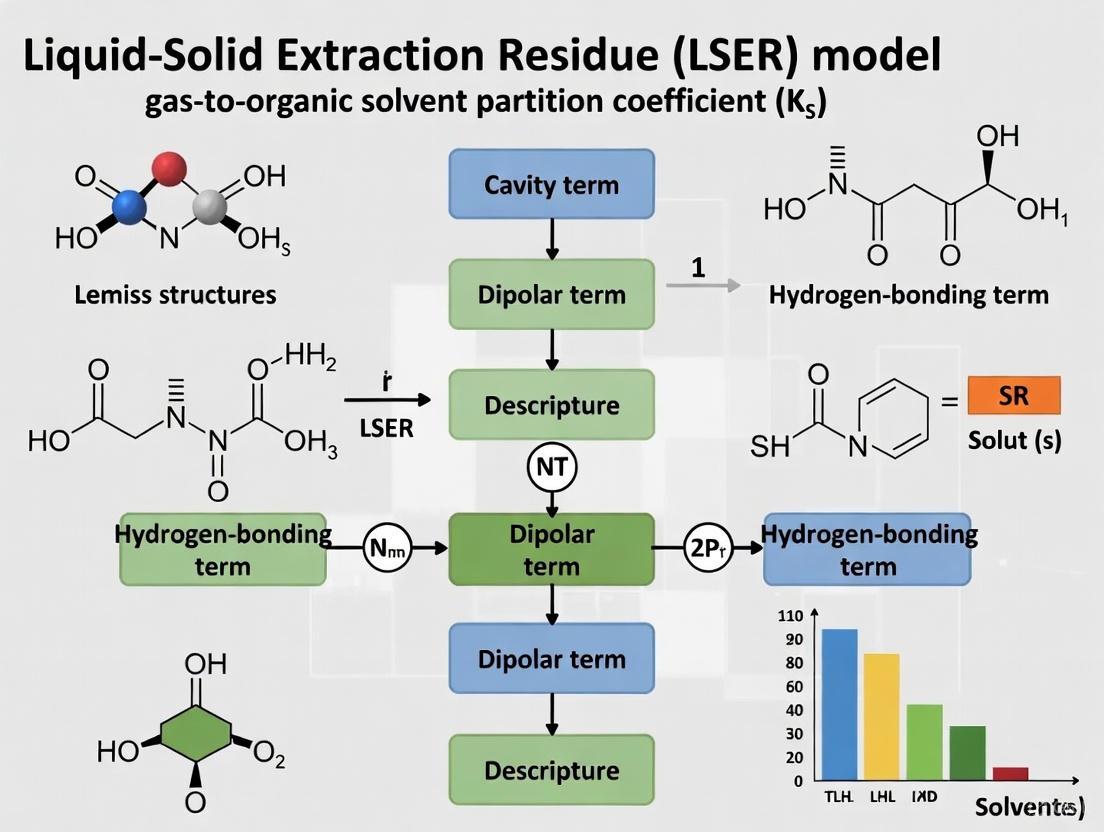
Visualizing the LSER Workflow and Solute-Solvent Interactions

The following diagram illustrates the logical workflow and the key solute-solvent interactions characterized by the LSER model.

LSER Model Workflow and Molecular Interactions

Successful application of the LSER model relies on a combination of experimental data, computational tools, and curated databases.

Table 2: Essential Research Tools for LSER Applications

Tool / Resource	Type	Function in LSER Research	Example / Source
Abraham Solute Descriptor Database	Database	Provides a curated set of experimentally derived solute descriptors (E, S, A, B, V, L) for thousands of compounds, essential for regression and prediction.	UFZ-LSER Database [9]
Abraham Solvent Coefficients	Dataset	A compiled set of solvent coefficients (c, e, s, a, b, v, l) for common organic solvents, required for predicting partition coefficients and solubilities.	Literature compilation by Acree et al. [9]
AbraLlama Models	AI Prediction Tool	Fine-tuned large language models (LLMs) that predict Abraham solute descriptors and modified solvent parameters directly from SMILES strings.	AbraLlama-Solute & AbraLlama-Solvent on Hugging Face [9]
Open Notebook Science Challenge	Data Repository	An open data collection of solubility measurements for organic compounds, used to determine new solute descriptors.	Royal Society of Chemistry sponsored project [7]
Quantum Chemical (QC) Software	Computational Tool	Performs calculations (e.g., COSMO-RS) to derive molecular charge densities and predict solvation energies, aiding in descriptor determination.	COSMO-RS implementations [6]
Random Forest Solvent Models	Predictive Model	Machine learning models that predict Abraham solvent coefficients for new organic solvents, extending the model's applicability.	Bradley et al. open models [10]

The deconstruction of the LSER solute descriptors (E, S, A, B, L, Vx) provides a powerful, quantitative framework for understanding and predicting solute behavior in gas-to-solvent partitioning. By following the detailed protocols for determining partition coefficients and solute descriptors, and by leveraging the modern computational tools and databases outlined in the Scientist's Toolkit, researchers can effectively apply the Abraham model to advance research in drug development, environmental chemistry, and chemical engineering. The ongoing integration of machine learning and quantum chemical calculations promises to further expand the accuracy and scope of this foundational model.

The Abraham solvation parameter model, or Linear Solvation Energy Relationship (LSER), is a powerful predictive tool in chemical, environmental, and pharmaceutical research, successfully correlating free-energy-related properties of a solute with its molecular descriptors [2]. The model's core principle rests on linear free energy relationships (LFERs), which quantitatively describe how the standard free energy change ( \Delta G^{0} ) of a solvation or partitioning process correlates with molecular interaction parameters [11]. For a solute transferring from the gas phase to an organic solvent, the process is quantified by the gas-to-organic solvent partition coefficient, ( KS ), through the fundamental LSER equation [2]: [ \log (KS) = ck + ekE + skS + akA + bkB + lkL ] Here, the solute is described by its molecular descriptors: ( Vx ) (McGowan’s characteristic volume), ( L ) (gas–hexadecane partition coefficient), ( E ) (excess molar refraction), ( S ) (dipolarity/polarizability), ( A ) (hydrogen bond acidity), and ( B ) (hydrogen bond basicity). The system's characteristics are captured by the solvent-specific coefficients ( ck ), ( ek ), ( sk ), ( ak ), ( bk ), and ( l_k ), which are determined via multiple linear regression of experimental data [2]. The very existence of this linearity, even for strong, specific interactions like hydrogen bonding, has been a subject of scientific inquiry, with recent work verifying its robust thermodynamic basis by combining equation-of-state solvation thermodynamics with the statistical thermodynamics of hydrogen bonding [2].

The Thermodynamic Basis of LSER Linearity

The Role of Free Energy and Enthalpy-Underscoring Linearity

The remarkable linearity observed in LSER models finds its foundation in the principles of thermodynamics. The quantitative relationships developed via theoretical derivation in physical chemistry are inherently robust and independent of the specific compounds studied [11]. The partition coefficient ( \log (KS) ) is directly proportional to the standard free energy change ( \Delta G^{0}{tr} ) for the solute transfer process ( \Delta G^{0}{tr} = -RT \ln KS ). This free energy change itself is a function of the corresponding standard enthalpy ( \Delta H^{0}{tr} ) and entropy ( \Delta S^{0}{tr} ) changes [11]. The LSER model effectively deconvolutes this overall ( \Delta G^{0}{tr} ) into contributions from distinct, independent types of intermolecular interactions, with each term in the LSER equation ( ekE, skS, akA, bkB, lkL ) representing a partial free energy contribution associated with a specific interaction mode [2] [11].

A major challenge has been understanding why these relationships remain linear despite the presence of strong, specific interactions like hydrogen bonding. Research confirms there is a solid thermodynamic basis for this LFER linearity. The combination of equation-of-state solvation thermodynamics with the statistical thermodynamics of hydrogen bonding verifies that the linearity holds because the LSER formalism effectively captures the free energy contributions of these interactions in a way that remains additive across diverse solute-solvent systems [2]. This linearity extends to other thermodynamic properties, such as solvation enthalpy ( \Delta HS ), which can be described by a similar linear equation [2]: [ \Delta HS = cH + eHE + sHS + aHA + bHB + lHL ] This equation allows for the extraction of enthalpic information on intermolecular interactions, providing a more detailed thermodynamic picture of the solvation process.

Key Molecular Descriptors and Intermolecular Interactions

Table 1: LSER Solute Descriptors and Their Physicochemical Significance

Descriptor	Symbol	Related Interaction Type	Thermodynamic Interpretation
McGowan's Characteristic Volume	( V_x )	Dispersion/Cavity Formation	Energy cost of creating a cavity in the solvent and the gain from dispersion forces.
Gas-Hexadecane Partition Coefficient	( L )	Dispersion Interactions	Free energy of solvation in an aliphatic hydrocarbon reference solvent.
Excess Molar Refraction	( E )	Polarizability from ( \pi )- and ( n )-electrons	Measures solute polarizability and its contribution to dispersion and polarization interactions.
Dipolarity/Polarizability	( S )	Dipolar & Polarization Interactions	Free energy contribution from dipole-dipole and dipole-induced dipole interactions.
Hydrogen Bond Acidity	( A )	Hydrogen Bond Donating Ability	Free energy contribution from the solute acting as a hydrogen bond donor (acid) to the solvent.
Hydrogen Bond Basicity	( B )	Hydrogen Bond Accepting Ability	Free energy contribution from the solute acting as a hydrogen bond acceptor (base) from the solvent.

Experimental Protocols for LSER Model Application

Protocol 1: Determination of Gas-to-Organic Solvent Partition Coefficients (( K_S )) Using Headspace Gas Chromatography (HSGC)

This protocol outlines the experimental determination of gas-liquid partition coefficients for neutral organic solutes, providing the primary data for constructing and validating LSER models [12].

1. Primary Reagents and Materials:

• Analyte Solutes: High-purity volatile organic compounds (e.g., alkanes, alcohols, ketones, aromatic compounds).
• Organic Solvents: Anhydrous solvents of high purity (e.g., n-hexadecane, n-octanol, chloroform) to cover a range of interaction types.
• Gas Chromatograph: Equipped with a flame ionization detector (FID) or mass spectrometer (MS).
• Headspace Vials: Sealed vials with PTFE/silicone septa.
• Gas-tight Syringes: For precise injection of headspace samples.

2. Procedure: 1. Sample Preparation: Prepare a series of headspace vials containing a known, constant volume of the organic solvent. Inject a range of microgram quantities of the analyte solute into the vials to establish a concentration series. Ensure vials are immediately sealed to prevent volatile loss [12]. 2. Equilibration: Place the prepared vials in a thermostated agitator (e.g., 25°C / 298.15 K) for a sufficient time to ensure equilibrium partitioning between the gas and liquid phases is achieved [12]. 3. Headspace Sampling: Using a gas-tight syringe, extract a defined volume of the equilibrated gas phase from the headspace of the vial. 4. GC Analysis: Inject the headspace sample into the GC system. Use an appropriate column (e.g., a non-polar capillary column) to separate the analyte. Record the peak area or height. 5. Calibration: Construct a calibration curve by analyzing headspace samples above a reference system (e.g., the pure analyte) or by using standard addition methods. 6. Data Calculation: The gas-to-solvent partition coefficient ( KS ) is calculated as ( KS = C{\text{solvent}} / C{\text{gas}} ), where ( C ) is the concentration in the respective phase at equilibrium, derived from the GC signal and the calibration curve [12].

3. Analysis and LSER Data Generation: 1. For each solute-solvent pair, perform multiple replicates to ensure precision. 2. Compile the log ( KS ) values for a wide range of chemically diverse solutes in the solvent of interest. 3. Use multiple linear regression analysis to fit the experimental log ( KS ) data against the known solute descriptors ( (E, S, A, B, L, Vx) ), thereby obtaining the solvent-specific coefficients ( (ck, ek, sk, ak, bk, l_k) ) for the LSER model [2] [12].

Protocol 2: In Silico Prediction of Polymer-Water Partition Coefficients using the UFZ-LSER Database

This protocol describes the use of a publicly available database to predict partition coefficients for neutral compounds, which is highly relevant for assessing the distribution of drug molecules or environmental contaminants [4] [13].

1. Primary Reagents and Materials:

• UFZ-LSER Database: Access the online database at https://www.ufz.de/lserd/ [4].
• Compound List: A list of neutral organic compounds for which predictions are needed.
• Solute Descriptors: Experimental or in silico predicted LSER solute descriptors (E, S, A, B, V, L) for the compounds of interest.

2. Procedure: 1. Database Navigation: - Access the UFZ-LSER database. The interface allows the calculation of various partitioning properties [4]. - Select the appropriate calculation module, such as "Calculate the sorbed concentration" or "Calculate the fraction of solute in the solvent" depending on the required output. 2. System Definition: - For polymer-water partitioning (e.g., Low-Density Polyethylene (LDPE)/Water), the database contains pre-defined LSER system parameters. For LDPE/water, the model is: log ( K_{i,\text{LDPE/W}} = -0.529 + 1.098E - 1.557S - 2.991A - 4.617B + 3.886V ) [13]. - If using a custom solvent system, the corresponding solvent coefficients must be available or determined first via Protocol 1. 3. Input of Solute Data: - Input the solute descriptors for the target compounds. The database contains a built-in chemical list, or users can input custom descriptor values [4]. 4. Calculation and Output: - Execute the calculation. The database will return the predicted partition coefficient (log P or log K) [4]. - Export the results for further analysis.

3. Analysis and Validation: - Benchmarking: For critical applications, validate the in silico predictions against a limited set of experimental data, if available. The LSER model for LDPE/water has been benchmarked with an independent validation set, yielding high accuracy (R² = 0.985, RMSE = 0.352) when using experimental solute descriptors [13]. - Domain of Applicability: Note that the model is only valid for neutral chemicals, and the domain of applicability for each descriptor should be considered [4].

Computational Workflow and Data Visualization

The following diagram illustrates the integrated experimental and computational workflow for developing and applying an LSER model, from data generation to prediction and validation.

The Scientist's Toolkit: Key Research Reagents and Materials

Table 2: Essential Materials and Resources for LSER-Based Research

Item/Resource	Function in LSER Research	Example/Specification
UFZ-LSER Database	A curated, publicly accessible database for obtaining solute descriptors and calculating partition coefficients for neutral compounds in various systems [4].	https://www.ufz.de/lserd/; Contains over 390,000 data points [4].
Reference Solvents	Used in experiments to determine solute descriptors or solvent coefficients. They cover a spectrum of interaction types.	n-Hexadecane (dispersion), n-Octanol (H-bonding), Chloroform (H-bond acidity), Diethyl Ether (H-bond basicity) [2] [12].
High-Purity Solutes	Chemically diverse analytes used to parameterize LSER models through measurement of their partition coefficients.	Linear/Branched Alkanes, Alcohols, Ketones, Ethers, Aromatic Compounds [12].
Headspace Gas Chromatograph (HSGC)	The primary analytical instrument for the accurate determination of gas-liquid partition coefficients without interference from interfacial adsorption [12].	System equipped with FID/MS detector and thermostated headspace autosampler.
Quantum-Chemical (QC) Descriptors	Molecular descriptors derived from computational chemistry that can be used to supplement or predict LSER parameters, aiding in the extension to compounds lacking experimental data [14].	Descriptors calculated via methods like COSMO-RS or other QC packages; sometimes referred to as QC-LSER descriptors [14].
Colorblind-Friendly Palette	A set of colors for creating accessible data visualizations and charts, ensuring interpretability for all researchers.	Palette of #d55e00, #cc79a7, #0072b2, #f0e442, #009e73 [15].
Hsd17B13-IN-29	Hsd17B13-IN-29, MF:C23H14Cl2N4O3, MW:465.3 g/mol	Chemical Reagent
Nisoldipine-d3	Nisoldipine-d3, MF:C20H24N2O6, MW:391.4 g/mol	Chemical Reagent

Understanding System Coefficients as Complementary Solvent Properties

Within the Linear Solvation Energy Relationship (LSER) framework for predicting gas-to-organic solvent partition coefficients (K_S), the system coefficients (e, s, a, b, l, c) are not merely fitting parameters. They represent the complementary properties of the solvent phase, quantitatively describing its capacity for various intermolecular interactions. This application note delineates the protocol for determining and interpreting these coefficients, framing them as essential descriptors for predicting solute partitioning in pharmaceutical and environmental research.

The Abraham solvation parameter model is a powerful tool for predicting a wide array of chemical, biomedical, and environmental processes [2]. For the gas-to-organic solvent partition coefficient (K_S), the model employs the following linear free-energy relationship (LFER) [16]:

log(K_S) = c + eE + sS + aA + bB + lL

In this equation, the capital letters (E, S, A, B, L) are solute descriptors—molecular properties that are intrinsic to the solute and remain constant across different systems [16]. In contrast, the lower-case letters (e, s, a, b, l, c) are the system coefficients (or solvent coefficients). These coefficients are complementary properties of the solvent phase. They are determined through multiple linear regression of experimental partition data for a diverse set of solutes with known descriptors and represent the solvent's capacity to participate in specific intermolecular interactions [2] [16]. The practical application of this model relies on the availability of both solute descriptors and pre-determined system coefficients for the solvent of interest.

Thermodynamic Interpretation of Coefficients

The LSER model is grounded in a cavity theory of solvation, where the process is divided into creating a cavity in the solvent, reorganizing the solvent, and establishing solute-solvent interactions [17]. The system coefficients in the log(K_S) equation are linearly related to the free energy of transfer from the gas phase to the solvent [17]. Each coefficient quantifies the complementary effect of the solvent on a specific interaction type:

• Cavity Formation and Dispersive Interactions: The l coefficient is primarily associated with the solvent's response to the cavity formation energy and dispersive (van der Waals) interactions, characterized by the solute's L descriptor (logarithmic hexadecane-air partition coefficient) [16].
• Polar Interactions: The s coefficient reflects the solvent's dipolarity/polarizability and its complementary interaction with the solute's dipolarity/polarizability (S descriptor) [16].
• Hydrogen-Bonding Interactions: The a and b coefficients describe the solvent's hydrogen-bond basicity and acidity, respectively. They interact complementarily with the solute's hydrogen-bond acidity (A descriptor) and basicity (B descriptor) [2] [16].
• Non-Specific Interactions: The e coefficient relates to the solvent's interaction with the solute's excess molar refraction (E descriptor) [16].

A significant advancement is the development of a single LSER equation that can predict partitioning between any two bulk phases, simplifying the application of the thermodynamic cycle and improving predictions for specific compound classes like highly fluorinated molecules [16].

Protocol for Determining System Coefficients

This protocol details the experimental and computational methodology for determining the system coefficients (e, s, a, b, l, c) for a new organic solvent.

Experimental Determination of Gas-Solvent Partition Coefficients (K_S)

Principle: The system coefficients for a solvent are derived by correlating experimentally measured log(K_S) values for a set of reference solutes with their known solute descriptors.

Materials & Equipment:

• Gas Chromatograph: Equipped with a flame ionization detector (FID) or mass spectrometer (MS).
• Capillary Column: Coated with the solvent of interest as the stationary phase.
• Reference Solutes: A training set of 30-50 compounds with known Abraham solute descriptors (E, S, A, B, L). The set must be chemically diverse, encompassing a wide range of polarity, hydrogen-bonding ability, and size.
• Syringe: For sample injection.
• Data Acquisition System: To record retention times.

Procedure:

• Column Preparation: Coat a deactivated capillary column with the solvent of interest, ensuring a uniform and stable stationary phase film to minimize adsorption effects [17].
• Dead Time Determination: Inject a non-retained compound (e.g., methane or air) at the desired temperature (commonly 25°C or other relevant temperatures) to determine the column's dead time (t_m).
• Retention Time Measurement: For each reference solute in the training set, inject a small sample onto the column and record its retention time (t_R). Ensure all measurements are conducted at the same, constant temperature.
• Calculate Capacity Factor: For each solute, calculate the capacity factor (k) using the formula: k = (t_R - t_m) / t_m [17].
• Calculate log(KS): Determine the gas-liquid partition coefficient, KS. For a capillary column, this can be related to the capacity factor and the phase ratio (Φ = VS / VM). The specific calculation may vary based on the chromatographic setup and available parameters [17].

Computational Regression for Coefficient Determination

Procedure:

• Data Compilation: Create a data matrix with the experimentally determined log(K_S) values for all reference solutes and their corresponding known solute descriptors (E, S, A, B, L).
• Multiple Linear Regression: Use statistical software (e.g., R, Python with scikit-learn) to perform a multiple linear regression. The model is: log(K_S) = c + eE + sS + aA + bB + lL
• Output Analysis: The output of the regression will provide the best-fit values for the system coefficients (e, s, a, b, l, c). The quality of the fit is typically assessed by the correlation coefficient (R²), standard error, and the significance (p-values) of each coefficient.

Data Presentation: Solvent-System Coefficients

The following table summarizes example system coefficients for different organic solvents, illustrating how these values reflect the chemical nature of the solvent. The coefficients a and b are particularly indicative of a solvent's hydrogen-bonding character.

Table: Exemplar System Coefficients for Selected Organic Solvents in the Gas-to-Solvent Partitioning LSER Equation [16]

Solvent	e	s	a	b	l	c
n-Hexadecane	0.000	0.000	0.000	0.000	1.000	0.000
Diethyl Ether	0.000	0.250	0.000	0.450	0.950	-0.300
Ethyl Acetate	0.000	0.620	0.000	0.450	0.900	-0.500
Methanol	0.000	0.400	0.300	0.500	0.800	-0.500
Water	0.000	0.600	1.000	0.200	0.500	-1.200

Note: The values in this table are illustrative examples. For actual research, coefficients should be sourced from comprehensive, peer-reviewed databases.

The Scientist's Toolkit: Essential Research Reagents & Materials

Table: Key Materials for LSER-Based Partition Coefficient Studies

Item	Function/Description
n-Hexadecane	A non-polar reference solvent for determining the solute's L descriptor and for calibrating GC systems [17].
Apolane-C87	A branched, high-molecular-weight alkane stationary phase for GC, allowing for the determination of log L for heavy, non-volatile compounds at elevated temperatures [17].
Reference Solute Training Set	A chemically diverse library of compounds with pre-established, high-quality Abraham solute descriptors for regression analysis [16].
Deactivated Capillary GC Columns	Inert columns that minimize adsorption of polar solutes onto the column surface, ensuring accurate measurement of partition coefficients [17].
LSER & PSP Databases	Freely accessible databases containing solute descriptors and system coefficients, which are rich sources of thermodynamic information [2].
Dat-IN-1	Dat-IN-1, MF:C29H34F2N2O2S, MW:512.7 g/mol
Dhodh-IN-25	Dhodh-IN-25, MF:C22H19ClF5N3O5, MW:535.8 g/mol

Visualizing the LSER Coefficient Determination Workflow

The following diagram illustrates the logical flow and sequence of steps from experimental setup to the final determination of the system coefficients.

Experimental Workflow for LSER Coefficient Determination

Visualizing the Conceptual Framework of LSER

This diagram deconstructs the LSER equation to show the complementary relationship between solute descriptors and solvent system coefficients in determining the overall partition coefficient.

LSER Conceptual Framework: Solute-Solvent Complementarity

The Significance of K_S in Pharmaceutical and Environmental Contexts

The Abraham solvation parameter model, also known as the Linear Solvation Energy Relationship (LSER), is a cornerstone predictive tool in chemical, environmental, and pharmaceutical research [2]. It provides a robust framework for understanding and quantifying the partitioning behavior of solutes between different phases. A fundamental parameter within this model is the gas-to-organic solvent partition coefficient, denoted as K_S. This coefficient describes the equilibrium distribution of a neutral compound between a gaseous phase and an organic solvent, providing direct insight into solute-solvent interactions [2].

The LSER model correlates free-energy-related properties, such as log KS, with a set of six empirically derived solute descriptors [2]. The governing equation for KS is expressed as:

log (K_S) = ck + ekE + skS + akA + bkB + lkL [2]

In this equation:

• K_S: Gas-to-organic solvent partition coefficient.
• E: Excess molar refraction.
• S: Solute dipolarity/polarizability.
• A: Solute hydrogen-bond acidity.
• B: Solute hydrogen-bond basicity.
• L: The logarithm of the gas–hexadecane partition coefficient at 298 K.
• ck, ek, sk, ak, bk, lk: System-specific coefficients (solvent descriptors) determined through multiple linear regression of experimental data.

The remarkable feature of this model is that the coefficients (e.g., ak, bk) are solvent-specific descriptors, reflecting the complementary properties of the solvent phase, while the variables (e.g., A, B) are solute-specific molecular descriptors [2]. This separation makes the LSER model a powerful tool for predicting partitioning behavior for a wide array of chemicals, including those for which experimental data are scarce.

LSER Fundamentals and K_S Equation Coeients

The predictive power of the K_S equation stems from its detailed accounting of different intermolecular interaction modes. Each term in the equation quantifies a specific contribution to the overall solvation energy.

Table 1: Interpretation of Coefficients and Descriptors in the log K_S Equation

Symbol	Name	Interpretation	Role in Solvation Energy
E	Excess Molar Refraction	Measures solute ability to interact with solvent via n- and π-electron pairs	ekE represents polarization interactions
S	Dipolarity/Polarizability	Measures solute ability to stabilize a neighboring charge or dipole	skS represents dipole-dipole and dipole-induced dipole interactions
A	Hydrogen-Bond Acidity	Measures solute ability to donate a hydrogen bond	akA represents the energy from solute-acid/solvent-base H-bonding
B	Hydrogen-Bond Basicity	Measures solute ability to accept a hydrogen bond	bkB represents the energy from solute-base/solvent-acid H-bonding
L	Gas-Hexadecane Partition Coefficient	Measures dispersion interactions and cavity formation energy	lkL represents the energy cost of forming a cavity in the solvent

The system constants (ck, ek, sk, ak, bk, lk) describe the solvent's properties. A positive system constant indicates that the corresponding solute property increases the partition coefficient K_S, favoring solvation in the liquid phase. For instance, a large positive ak value for a solvent indicates that it is a strong hydrogen-bond base and will strongly solvate solutes with high hydrogen-bond acidity (A) [2].

Applications in Pharmaceutical and Environmental Sciences

The LSER model for K_S is indispensable in pharmaceutical development and environmental risk assessment, where predicting the partitioning behavior of organic compounds is critical.

Application Notes: K_S in Pharmaceutical Development

In the pharmaceutical and medical device industries, the Abraham model is widely applied in extractables and leachables (E&L) studies to ensure product safety [1]. Key applications include:

• Evaluation of Drug Product Simulating Solvents: K_S values and LSER models help select and validate solvents that simulate the chemical properties of a drug product for extraction studies, ensuring that laboratory tests accurately predict the leaching potential from container closure systems or medical devices [1].
• Prediction of Chromatographic Retention: LSER models can correlate and predict the retention behavior of E&L compounds in chromatographic systems. This application aids in the identification of unknown compounds, a major challenge in E&L profiling [1].
• Understanding Solvent Extraction Power: The model allows scientists to rationally select extraction solvents for polymeric materials used in medical devices and packaging by quantitatively understanding the specific interactions (dipolarity, hydrogen-bonding, etc.) that govern a solvent's extraction efficiency toward a target analyte [1].

Application Notes: K_S in Environmental Risk Assessment

Environmental risk assessment (ERA) for human pharmaceuticals is a growing regulatory focus worldwide. The LSER model, particularly through K_S and related partition coefficients, plays a vital role in this process.

• Predicting Environmental Fate and Transport: Partition coefficients are key parameters in mass transport models that predict the distribution and concentration of pharmaceutical residues in environmental compartments such as water, soil, and air [13]. For example, a robust LSER model has been established for the partition coefficient between low-density polyethylene (LDPE) and water, which is critical for assessing the sorption of contaminants to plastic materials in the environment [13].
• Regulatory Compliance: The revised "Guideline on the Environmental Risk Assessment of Medicinal Products for Human Use" mandates a comprehensive evaluation of a pharmaceutical's environmental impact [18]. LSER models provide a reliable, predictive tool to generate the necessary partitioning data, especially for compounds in the early stages of development where experimental data may be lacking. The ability of LSERs to predict partition coefficients for a "wide set of chemically diverse compounds" makes them exceptionally valuable for this purpose [13].
• Prioritization of Compounds: LSER-predicted K_S values can help prioritize which pharmaceuticals warrant more extensive and costly experimental testing based on their potential to persist, bioaccumulate, or partition into sensitive environmental compartments [18].

Experimental Protocols

This section provides a detailed methodology for determining the gas-to-organic solvent partition coefficient (K_S) and its subsequent use in developing and applying LSER models.

Protocol 1: Determination of log K_S via Headspace Gas Chromatography

Objective: To experimentally determine the gas-to-organic solvent partition coefficient (K_S) for a volatile solute using static headspace gas chromatography (HS-GC).

Principle: The concentration of a solute in the headspace gas above a solvent is measured at equilibrium. The partition coefficient is calculated from the relative concentrations in the gas and solvent phases.

Table 2: Key Research Reagent Solutions for K_S Determination

Reagent/Material	Function	Critical Specifications
Organic Solvent	Partitioning phase	High purity (e.g., HPLC grade), low volatility, known water content
Analyte (Solute)	Compound whose K_S is being measured	High purity, volatile and stable under experimental conditions
Internal Standard	Reference for GC quantification	Chemically similar, non-interfering, and known partitioning behavior
Gas-Tight Syringes	Sampling headspace and liquid	Heated syringe to prevent condensation during transfer
Headspace Vials	Contain equilibrated system	Certified with precise volume, sealed with PTFE/silicone septa

Procedure:

• Solution Preparation: Precisely prepare a stock solution of the analyte in the organic solvent. Introduce a known aliquot of this solution into a headspace vial, ensuring there is significant headspace. Seal the vial immediately with a crimp cap.
• Equilibration: Place the sealed vials in a thermostated HS-GC autosampler and allow them to equilibrate at a constant temperature (e.g., 25°C ± 0.1°C) with continuous agitation for a time sufficient to reach equilibrium (typically 30-60 minutes).
• Headspace Sampling & GC Analysis: Using a heated gas-tight syringe, extract a defined volume of the headspace vapor from the equilibrated vial and inject it into the gas chromatograph. Use an appropriate detector (e.g., FID).
• Calibration: Construct a calibration curve by analyzing headspace samples above standard solutions of the analyte with known concentrations.
• Data Analysis: Calculate the concentration of the analyte in the gas phase (Cgas) directly from the GC peak area and the calibration curve. The concentration in the solvent phase (Csolv) can be determined by mass balance from the initial amount added and the measured amount in the headspace. The partition coefficient is then calculated as KS = Csolv / Cgas. The logarithm of this value, log KS, is used in LSER analysis.

Protocol 2: Developing a Solvent-Specific LSER Model

Objective: To derive the system constants (ck, ek, sk, ak, bk, lk) for a specific organic solvent.

Principle: By measuring log K_S for a training set of solutes with known and diverse molecular descriptors (E, S, A, B, L), the system constants for the solvent can be determined via multiple linear regression.

Procedure:

• Solute Selection: Carefully select a training set of 30-50 solutes that collectively exhibit a wide range of E, S, A, B, and L values. The diversity is critical for a robust and meaningful model.
• Data Collection: For each solute in the training set, determine the log K_S value in the target solvent using Protocol 1 or obtain reliable data from literature. Obtain the solute's molecular descriptors (E, S, A, B, L, Vx) from a curated database, such as the UFZ-LSER database [4].
• Multiple Linear Regression: Input the matrix of solute descriptors (independent variables) and the experimental log K_S values (dependent variable) into a statistical software package capable of multiple linear regression.
• Model Validation: Validate the derived LSER equation by predicting log K_S for a separate validation set of solutes not included in the training set. Compare the predicted values against experimental results. A robust model is indicated by high R² values (>0.95) and low root mean square error (RMSE) [13].

Data Presentation and Analysis

The following tables present LSER model coefficients and predictive performance data to illustrate practical applications.

Table 3: Exemplary LSER System Constants for log K_S in Various Solvents

Solvent	ck	ek	sk	ak	bk	lk	R²	n
n-Hexadecane	-0.23	0.00	0.00	0.00	0.00	1.00	0.999	150
Diethyl Ether	-0.32	0.25	0.42	0.00	1.05	0.85	0.995	120
Ethyl Acetate	-0.21	0.38	1.17	0.00	1.84	0.74	0.992	130
Methanol	-0.17	0.41	0.60	3.68	1.89	0.52	0.987	140

Table 4: Benchmarking of an LSER Model for LDPE/Water Partitioning [13]

Dataset	Number of Compounds (n)	Determination Coefficient (R²)	Root Mean Square Error (RMSE)	Notes
Training Set	104	0.991	0.264	Model development
Validation Set (Exp. Descriptors)	52	0.985	0.352	Independent model validation
Validation Set (Pred. Descriptors)	52	0.984	0.511	Real-world scenario for new chemicals

The Scientist's Toolkit

Table 5: Essential Resources for LSER and K_S Research

Tool / Resource	Description	Utility in K_S Research
UFZ-LSER Database	A freely accessible, curated database of LSER solute descriptors and calculation tools [4].	Primary source for obtaining solute descriptors (E, S, A, B, L, Vx) needed for predictions.
Headspace GC System	Gas chromatograph equipped with a static headspace autosampler.	Core experimental apparatus for the accurate determination of gas-to-solvent partition coefficients (K_S).
Statistical Software	Package capable of multiple linear regression (e.g., R, Python with scikit-learn).	Essential for deriving system constants from experimental log K_S data and validating model performance.
QSPR Prediction Tools	In-silico tools for predicting LSER solute descriptors from chemical structure alone.	Enables K_S estimation for novel compounds for which experimental descriptors are not available [13].
GLP-Certified Laboratory	Laboratory operating under Good Laboratory Practice standards.	Required for generating environmental risk assessment (ERA) data for regulatory submission to agencies like the EMA and FDA [18].
Notrilobolide	Notrilobolide, MF:C26H36O10, MW:508.6 g/mol	Chemical Reagent
Bace1-IN-14	Bace1-IN-14, MF:C26H20FN3O, MW:409.5 g/mol	Chemical Reagent

The gas-to-organic solvent partition coefficient, KS, as formalized within the Abraham LSER model, is a parameter of profound significance. Its power lies in a rigorous thermodynamic foundation that decouples solute properties from solvent properties, enabling the accurate prediction of partitioning behavior for diverse compounds [2]. As demonstrated, the application of KS and LSER models is critical in pharmaceutical development, particularly for E&L studies and medical device characterization [1], and in environmental science for forecasting the fate and impact of pollutants and pharmaceuticals [18] [13]. The ongoing development of curated databases and predictive tools ensures that the LSER approach will remain a vital, evolving resource for researchers and regulators committed to product safety and environmental health.

From Theory to Practice: Determining Descriptors and Applying the LSER Model

Experimental Methods for Determining log L16 Using Gas Chromatography

Within the Linear Solvation Energy Relationship (LSER) model, the log L16 solute descriptor is a fundamental parameter, defined as the logarithm of the gas-hexadecane partition coefficient at 298 K [2] [19]. It quantifies a solute's capacity for dispersion interactions and the energy required for cavity formation within the solvent matrix, serving as a key characteristic in the Abraham solvation parameter model [20] [17]. Accurate determination of log L16 is crucial for predicting thermodynamic properties and molecular interactions in various chemical, biomedical, and environmental processes [2] [21]. This Application Note details validated chromatographic methods for the precise experimental measurement of log L16, providing essential protocols for researchers engaged in LSER-based studies of gas-to-organic solvent partition coefficients (K_S).

Theoretical Background and Significance

The LSER model for characterizing solvent-solute interactions utilizes two primary equations for partitioning processes. For gas-to-solvent partitioning, the model is expressed as:

log (K_S) = c_k + e_kE + s_kS + a_kA + b_kB + l_kL [2] [21]

In this equation, the capital letters (E, S, A, B, L) represent solute-specific molecular descriptors, while the lower-case letters are system-specific coefficients that reflect the complementary properties of the solvent phase. The L descriptor, and specifically log L¹⁶, characterizes the solute's partitioning into n-hexadecane, a solvent chosen for its ability to engage almost exclusively in non-specific, predominantly dispersive interactions [20] [19]. The determination of log L16 is therefore a critical first step in characterizing a solute's complete set of LSER descriptors, as it anchors the scale for dispersion interactions and cavity formation [17].

Research Reagent Solutions

The following table catalogues essential materials and their specific functions in the experimental determination of log L16.

Table 1: Key Research Reagents and Materials for log L16 Determination

Material/Reagent	Function and Critical Specifications
n-Hexadecane Stationary Phase	Reference partitioning phase for defining log L16; high purity (>99%) is essential to minimize polar interactions [22] [17].
Squalane Packed Columns	A surrogate non-polar stationary phase for log L16 determination; requires correction for interfacial adsorption at the liquid-solid interface [22] [23].
Poly(methyloctylsiloxane) Columns	Immobilized open-tubular column phase; less cohesive with no hydrogen-bond basicity, suitable for a wider temperature range [22] [23].
Apolane-87 (C87H176) Stationary Phase	A branched, high-molecular-weight alkane for studying high-boiling compounds; stable at temperatures up to 550 K [17].
Inert Gas (Helium or Nitrogen)	Serves as the mobile phase (carrier gas) in GC systems; must be high-purity to avoid detector noise and baseline drift [24].

Methodologies and Experimental Protocols

Core Principles and Thermodynamic Basis

The chromatographic determination of log L16 is based on measuring the gas-liquid partition coefficient (K_L). The retention factor (k) of a solute is directly related to K_L and the phase ratio (Φ) of the column:

K_L = k / Φ [17]

The log L16 value is then the logarithm of this partition coefficient determined specifically on an n-hexadecane stationary phase at 25°C. The process of solvation in gas-liquid chromatography is interpreted through a three-step cavity theory: (1) creation of a solute-sized cavity in the solvent (endoergic), (2) reorganization of solvent molecules, and (3) establishment of solute-solvent interactions (exoergic) [20] [17]. The retention factor is a direct measure of the overall Gibbs energy change for this solvation process.

Protocol 1: Determination on n-Hexadecane Packed Columns

This protocol outlines the direct measurement of log L16 using custom-packed GC columns.

• Column Preparation: Pack a stainless-steel or glass column (e.g., 1-2 m length) with an inert diatomaceous earth support coated with 15-20% (m/m) n-hexadecane stationary phase. A high phase loading is critical to minimize the contribution of interfacial adsorption on the support surface [22] [17].
• Instrument Calibration: Precisely determine the column void time (t_M) using a non-retained compound (e.g., methane or air). Calculate the phase ratio (Φ) from the known volumes of the stationary (V_S) and mobile (V_M) phases [17].
• Retention Measurement: Inject the solute of interest and record its retention time (t_R). The retention factor is calculated as k = (t_R - t_M) / t_M. The partition coefficient is K_L = k / Φ. The value of log L16 is log K_L after correction to 25°C [17].
• Temperature Control and Adsorption Correction: Conduct measurements isothermally within the 80-120°C temperature range to optimize efficiency and reduce adsorption effects. For the most accurate results, the gas-liquid partition coefficient should be used as the model variable to correct for any residual temperature-dependent interfacial adsorption, allowing log L16 to be estimated to within ± 0.026 log units [22].

Protocol 2: Determination Using Poly(methyloctylsiloxane) Capillary Columns

This protocol utilizes a more robust, commercially available stationary phase as a surrogate system.

• Column Selection: Use a capillary column coated with an immobilized film of poly(methyloctylsiloxane). This phase is preferred over poly(dimethylsiloxane) due to its lower cohesion and lack of hydrogen-bond basicity, making it more suitable for log L16 determination [22] [23].
• Relative Retention Method: Since directly determining the exact mass of stationary phase in a capillary column is difficult, use a relative method. The partition coefficient for the solute at temperature T can be related to the known partition coefficient of a reference compound (e.g., n-hexane) at a specific temperature [17]. The relationship is derived from the linear correlation of partition coefficients at different temperatures for a given stationary phase.
• Data Interpretation: A single-column estimation of log L16 over the temperature range 60-140°C is possible with an error of ±0.05–0.09 log units. Note: This method requires prior knowledge of the solute's dipolarity/polarizability (S) descriptor to avoid significant errors for polar compounds [22].

Protocol 3: Determination for High-Boiling Compounds Using Temperature Gradients

For compounds less volatile than n-hexadecane, isothermal measurement at 25°C is impractical. Temperature Gradient Gas Chromatography (TGGC) offers a solution.

• System Setup: Utilize a GC system equipped for precise temperature programming. A column with a highly retentive non-polar phase like Apolane-87 is recommended for its thermal stability [19] [17].
• Linear Temperature-Programmed Retention Index (LTPRI): Within a homologous series, a linear relationship exists between the logarithm of the distribution coefficient (log K) and the LTPRI, which is calculated from retention times during a temperature ramp [19].
• Calibration and Prediction: Establish a calibration curve by measuring the LTPRI of compounds with known log L16 values. The log L16 for an unknown solute can then be predicted from its measured LTPRI using this calibration curve. This method also allows for the estimation of vapor pressures of high-boiling compounds [19].

The following workflow diagram illustrates the decision process for selecting the appropriate experimental protocol.

Data Analysis and Comparison of Methodologies

The following table summarizes the performance characteristics of the primary chromatographic methods for determining log L16, enabling researchers to select the most appropriate protocol for their needs.

Table 2: Comparison of Chromatographic Methods for log L16 Determination

Method	Typical Stationary Phase	Temperature Range	Estimated Accuracy	Key Advantages	Key Limitations
Direct Packed Column	n-Hexadecane (15-20% loading)	80-120 °C	± 0.026 log units [22]	Direct measurement; minimal model assumptions.	Requires custom-packed column; adsorption corrections needed.
Surrogate Capillary Column	Poly(methyloctylsiloxane)	60-140 °C	± 0.05 - 0.09 log units [22]	Uses robust commercial columns; wider temp range.	Requires solute's S descriptor for polar compounds [22].
Temperature Gradient (TGGC)	Apolane-87	Programmable	Varies with calibration [19]	Applicable to high-boiling, non-volatile compounds.	Indirect method; requires calibration with known compounds.

The accurate experimental determination of the log L16 solute descriptor is a foundational activity in the application of the LSER model. The chromatographic protocols detailed herein—utilizing packed n-hexadecane columns, surrogate poly(methyloctylsiloxane) capillary columns, and temperature-gradient methods for high-boiling compounds—provide researchers with a robust toolkit. The selection of the optimal method depends on the volatility of the solute, available instrumentation, and the required precision. By carefully applying these protocols, scientists can generate high-quality log L16 data essential for reliable predictions of gas-to-organic solvent partition coefficients and other thermodynamic properties in drug development and environmental research.

Computational and Predictive Approaches for Non-Volatile Solute Descriptors

Within the framework of Linear Solvation Energy Relationship (LSER) research for gas-to-organic solvent partition coefficients (K~S~), a significant challenge arises when characterizing non-volatile solutes. For such compounds, direct experimental determination of solute descriptors, particularly the L descriptor (the logarithmic hexadecane/air partition coefficient at 298 K), is often impossible via conventional gas chromatography (GC) methods at standard temperatures [25] [17]. This application note details established and emerging computational and predictive methodologies designed to overcome this limitation, enabling the reliable estimation of a complete set of Abraham solute descriptors for non-volatile compounds essential for environmental fate and drug distribution modeling.

The LSER model for gas-to-organic solvent partitioning is described by the equation [2]: log (K~S~) = c~k~ + e~k~E + s~k~S + a~k~A + b~k~B + l~k~L Here, the capital letters (E, S, A, B, L) represent the solute's molecular descriptors, while the lowercase letters are system constants characteristic of the solvent phase. The inability to determine L for non-volatile solutes creates a critical gap in this predictive framework.

Computational & Predictive Methodologies

Two parallel, complementary strategies have been developed to address the descriptor gap for non-volatile solutes: one based on extrapolative experimental techniques and the other on quantum chemical computations.

Chromatographic Extrapolation and Predictive Modeling

For compounds that are slightly volatile or have low volatility, a practical experimental approach involves measuring retention factors at elevated temperatures where analysis is feasible, followed by extrapolation to the target temperature of 298 K [25] [17].

A key technique utilizes apolane (C~87~H~176~) as a stationary phase. This branched alkane is stable at high temperatures (up to 550 K), allowing for the measurement of gas-apolane partition coefficients (log L~87~) for heavy compounds [17]. A linear correlation between log L~87~ and the desired log L~16~ has been demonstrated, enabling the estimation of L descriptors for non-volatile solutes [17]. The workflow for this method is integrated into the protocol below.

For completely non-volatile compounds, predictive methods become necessary. Research indicates that log L~16~ can be estimated for siloxanes and other organosilicon compounds by leveraging established LSER models that predict various physicochemical properties (e.g., vapor pressure, aqueous solubility) from their descriptors [25]. This suggests that once a foundational set of descriptors is known for a compound class, predictive models can be generalized for other members.

Quantum Chemical (QM) Approaches

Quantum mechanical methods provide a fundamental, non-experimental path to obtaining solute descriptors and partition coefficients. These approaches calculate the solvation energy (ΔG~solv~) in different solvents of interest (e.g., hexadecane, water, octanol) from first principles [26].

The calculated ΔG~solv~ values are directly related to the partition coefficients required for descriptor determination or can be used to parameterize the LSER equations directly [26] [27]. A significant advantage of QM methods is their ability to model complex molecules, including modern drug molecules, which are often difficult to handle experimentally due to legal restrictions or complex molecular structures [26]. Studies have successfully calculated log K~OW~, log K~OA~, log K~AW~, and log K~HdA~ (L) for diverse drug molecules in this way [26].

Table 1: Comparison of Approaches for Non-Volatile Solute Descriptor Determination

Methodology	Fundamental Principle	Key Advantage	Primary Limitation
Chromatographic Extrapolation	Measurement of retention factors at high temperature followed by extrapolation to 298 K [17].	Based on empirical data, high precision for semi-volatile compounds.	Requires the compound to be sufficiently volatile at elevated temperatures.
Predictive LFER Modeling	Uses known descriptors from a compound class to predict descriptors for similar, non-volatile compounds [25].	Bypasses experimentation entirely; useful for homologues.	Accuracy depends on the model and the similarity between the target and reference compounds.
Quantum Chemical Calculation	Computational calculation of solvation free energies in different phases to derive partition coefficients and descriptors [26].	Universally applicable, no experimental hurdles; suitable for novel/regulated compounds.	Requires significant computational resources and expert knowledge.

Experimental Protocol: Determination of log L~16~ for Semi-Volatile Compounds

This protocol describes the procedure for estimating the log L~16~ descriptor using a high-temperature apolane stationary phase, based on established chromatographic methods [25] [17].

Materials and Equipment

Table 2: Research Reagent Solutions and Essential Materials

Item Name	Function/Application
Apolane-coated Capillary GC Column (C~87~H~176~ stationary phase)	High-temperature stationary phase for determining gas-apolane partition coefficients (log L~87~) [17].
n-Hexane Standard	Reference compound for determining dead time and establishing relative retention [17].
n-Hexadecane	Reference non-polar stationary phase; the definition of the L descriptor (log K~HdA~) [25] [17].
GC-MS System	Equipped with an autosampler and temperature-programmable injector for precise retention time measurement [27].

Step-by-Step Procedure

• Column Preparation: Install a capillary GC column coated with apolane (C~87~H~176~). Ensure the column is conditioned according to the manufacturer's specifications.
• Dead Time (t~0~) Determination: Inject a small volume of air or methane and record the retention time of the argon peak (m/z 40) or the solvent front. This is the column dead time, t~0~ [27].
• n-Hexane Calibration: Inject n-hexane at the same high temperature (T') used for the solute analysis. Record its retention time (t~R,hex~) and calculate its partition coefficient on apolane at T' using established data or methods [17].
• Solute Analysis: Dissolve the target semi-volatile solute in a suitable volatile solvent (e.g., acetone). Inject the solution onto the apolane column at a temperature (T) high enough to produce a measurable retention time. Record the solute's retention time (t~R~).
• Retention Factor Calculation: For the solute and for n-hexane, calculate the retention factor, k, using the formula: k = (t~R~ - t~0~) / t~0~ [17] [27].
• Partition Coefficient Estimation: The gas-apolane partition coefficient for the solute at temperature T (log L~87,T~) can be found relative to n-hexane. A general relationship is used [17]: log L~X,T~ = log k~X,T~ + log L~Ref,T'~ + log (V~M~/V~S~) where L~Ref,T'~ is the known partition coefficient of the reference compound (n-hexane) at a specific temperature.
• Extrapolation to log L~16~: Utilize the established linear correlation between log L~87~ (determined at temperature T) and the target log L~16~ (at 298 K) to obtain the final L descriptor for the solute [17].

Diagram 1: Experimental workflow for determining the L descriptor for semi-volatile solutes using high-temperature gas chromatography.

Quantum Chemical Calculation Protocol

This protocol outlines the general steps for calculating the L descriptor and other solute parameters using quantum chemical methods, as applied in environmental and pharmaceutical research [26] [27].

• Software: Quantum chemical software packages (e.g., Gaussian, ORCA, COSMOlogic suite).
• Method: Density Functional Theory (DFT) with appropriate functionals (e.g., B3LYP) and basis sets (e.g., 6-311+G(d,p)).
• Solvation Model: A continuum solvation model such as COSMO-RS (Conductor-like Screening Model for Real Solvents) or SMD (Solvation Model based on Density).

Step-by-Step Procedure

• Geometry Optimization: Generate a 3D structure of the target molecule and perform a quantum chemical geometry optimization in the gas phase to find its most stable conformation.
• Frequency Calculation: Perform a frequency calculation on the optimized structure to confirm it is a true minimum (no imaginary frequencies) and to obtain thermodynamic corrections.
• Solvation Energy Calculations: Calculate the solvation free energy (ΔG~solv~) for the molecule in various phases:
  • n-Hexadecane: ΔG~solv,hd~
  • Air/Gas Phase: Effectively zero by definition.
  • (Optional) Water and octanol for other descriptors.
• Partition Coefficient Calculation: The hexadecane/air partition coefficient (K~HdA~) is related to the solvation free energy: log K~HdA~ (L) = -ΔG~solv,hd~ / (RT ln(10)) where R is the gas constant and T is the temperature (298 K).
• Descriptor Validation: Compare the predicted partition coefficients (e.g., log K~OW~) for which some experimental or QSAR data might exist to assess the plausibility of the QM results [26].

Table 3: Key Solute Descriptors and their Determination Methods

Solute Descriptor	Molecular Property	Determination Method for Non-Volatiles
L	Gas–hexadecane partition coefficient	Calculation from ΔG~solv~ in n-hexadecane via QM methods [26] or extrapolation from high-T GC [17].
V	McGowan's characteristic molar volume	Calculation by summation of atom volumes and bond contributions; trivial from structure [25].
E	Excess molar refraction	Calculation from characteristic volume V and refractive index (experimental or estimated) [25].
S	Dipolarity/Polarizability	Determined from GC on polar stationary phases or liquid-liquid partitions, often requiring inversion of LSER equations [25].
A & B	Hydrogen-Bond Acidity/Basicity	Determined from liquid-liquid distribution in totally organic biphasic systems (e.g., n-hexane-acetonitrile) [25] or via QM-based methods.

The accurate prediction of environmental transport and biological distribution of non-volatile compounds using LSER models depends critically on the availability of reliable solute descriptors. The methodologies outlined herein—chromatographic extrapolation and quantum chemical calculation—provide robust, complementary pathways for obtaining the essential L descriptor and other parameters that are inaccessible by standard experiments. The choice between these methods depends on the specific compound, available instrumentation, and computational resources. The integration of these computational and predictive approaches ensures the continued applicability and expansion of the LSER framework to complex, non-volatile organic compounds in environmental and pharmaceutical sciences.

Accessing and Utilizing the UFZ-LSER Database for System Coefficients

The UFZ-LSER database serves as a critical repository for solvation parameters and system coefficients essential for applying Linear Solvation Energy Relationships (LSERs). For research focused on predicting the gas-to-organic solvent partition coefficient (K_S), this database provides the experimentally derived system constants that quantify a solvent's capacity for various types of intermolecular interactions [2]. The Abraham LSER model, which underpins this database, describes K_S using the following general equation, where the capital letters represent solute-specific molecular descriptors and the lowercase letters represent the solvent-specific system coefficients obtainable from the database [2]:

log (K_S) = c_k + e_k*E + s_k*S + a_k*A + b_k*B + l_k*L

This equation allows researchers to predict partition coefficients for neutral compounds based on a set of six molecular descriptors characterizing their volume, polarity, and hydrogen-bonding capabilities [2] [28]. The UFZ-LSER database is freely accessible and represents a wealth of thermodynamic information validated through extensive experimental measurements, making it particularly valuable for drug development professionals seeking to understand compound solubilization and distribution [29] [30].

Accessing System Coefficients from the UFZ-LSER Database

Database Navigation and Interface

The UFZ-LSER database is hosted by the Helmholtz Centre for Environmental Research-UFZ and is accessible online. The interface provides multiple calculation modules, including those for biopartitioning, sorbed concentration, and extraction efficiencies [29]. For researchers investigating K_S, the core functionality lies in the database's ability to provide the system coefficients (c_k, e_k, s_k, a_k, b_k, l_k) for a wide range of organic solvents.

The main page presents a list of available chemicals and solvents, from which users can select compounds relevant to their research. The database includes common organic solvents such as octanol, hexane, ethyl acetate, and chloroform, among many others [29]. The web interface allows for direct input of parameters and retrieves calculated results dynamically.

Step-by-Step Protocol for Retrieving System Coefficients

• Access the Database: Navigate to the official UFZ-LSER database website.
• Select Calculation Type: Choose the appropriate module for your partitioning needs. For K_S calculations, this typically involves options related to gas-to-solvent partitioning.
• Choose Solvent System: Select the organic solvent(s) of interest from the provided list. The database contains numerous pre-defined solvents with curated system coefficients.
• Input Solute Parameters: If calculating specific partition coefficients, input the solute's molecular descriptors (E, S, A, B, V, L). Alternatively, the database can be queried solely for the solvent system coefficients themselves.
• Execute Calculation: Run the calculation to obtain the results. The output will include the partition coefficient or the system coefficients used in the LSER equation.
• Cite the Database: Properly acknowledge the source using the recommended citation format: "Ulrich, N., Endo, S., Brown, T.N., Watanabe, N., Bronner, G., Abraham, M.H., Goss, K.-U., UFZ-LSER database v 3.2.1 [Internet], Leipzig, Germany, Helmholtz Centre for Environmental Research-UFZ. 2017" [29].

Table: LSER Molecular Descriptors and their Physical Significance

Descriptor	Symbol	Physical Significance
McGowan's Characteristic Volume	V_x	Molecular size & cavity formation energy
Gas-Hexadecane Partition Coefficient	L	Dispersion interactions
Excess Molar Refraction	E	Polarizability due to π- or n-electrons
Dipolarity/Polarizability	S	Dipolarity & polarizability interactions
Hydrogen Bond Acidity	A	Solute's hydrogen bond donor ability
Hydrogen Bond Basicity	B	Solute's hydrogen bond acceptor ability

Experimental Protocol for Determining Gas-to-Organic Solvent Partition Coefficients (K_S)

Computational Determination of K_S Using LSERs

This protocol details the use of UFZ-LSER database coefficients to computationally predict K_S values for neutral organic compounds, a key parameter in pharmaceutical distribution studies.

Materials and Reagents:

• UFZ-LSER Database: Primary source for solvent system coefficients [29].
• Solute Descriptors: Set of six Abraham parameters (E, S, A, B, V, L) for the target solute.
• Calculation Software: Standard spreadsheet software or computational scripting environment.

Procedure:

• Retrieve Solvent Coefficients: Access the UFZ-LSER database and identify the system coefficients for your target organic solvent. These coefficients are specific to the gas-to-solvent partitioning process described by Equation (2) in the introduction [2].
• Obtain Solute Descriptors: Acquire the six molecular descriptors for your solute compound. These can be sourced from experimental measurements or predicted using Quantitative Structure-Property Relationship (QSPR) tools if experimental data is unavailable [31].
• Apply LSER Equation: Substitute the solvent system coefficients and solute molecular descriptors into the standard LSER equation for K_S: log(K_S) = c_k + e_k*E + s_k*S + a_k*A + b_k*B + l_k*L
• Calculate and Validate: Perform the calculation to obtain log(K_S). For validation, compare predicted values against experimental data for compounds with known partition coefficients, if available.

Workflow Visualization

The following diagram illustrates the computational workflow for determining K_S using the UFZ-LSER database:

Advanced Applications and Methodological Considerations

Research Applications and Case Studies

The LSER approach facilitated by the UFZ-LSER database has proven valuable in diverse research contexts:

• Micelle Partitioning: LSER models have been successfully developed to predict the partitioning of neutral chemicals into polysorbate 80 (PS 80) micelles, a system relevant to pharmaceutical formulation. The resulting model demonstrated excellent predictive capability (R² = 0.969) across 112 chemically diverse compounds, outperforming simple log P-based models [30].
• Polymer-Water Partitioning: LSERs provide accurate predictions for partition coefficients between low-density polyethylene (LDPE) and water (R² = 0.991, RMSE = 0.264 for n=156 compounds). This application is particularly important for predicting leachables from pharmaceutical packaging materials [31].
• Solvent Characterization: Principal Component Analysis (PCA) of gas-liquid partition coefficients for alkane solutes in organic solvents has confirmed that two principal factors adequately describe the partitioning behavior, validating the fundamental LSER approach for characterizing solvent properties [12].

The Scientist's Toolkit: Essential Research Reagents and Materials

Table: Key Resources for LSER-Based Partition Coefficient Research

Resource	Function/Description	Relevance to KS Determination
UFZ-LSER Database	Curated repository of solvent system coefficients and solute descriptors [29]	Primary source for obtaining the system-specific constants (ek, sk, ak, bk, l_k)
Abraham Solute Descriptors	Set of six molecular parameters (E, S, A, B, V, L) characterizing solute properties [2]	Essential inputs describing the compound of interest for the LSER equation
QSPR Prediction Tools	Computational methods for predicting solute descriptors when experimental values are unavailable [31]	Enables model application to compounds without experimentally measured descriptors
Polysorbate 80 Micelles	Common surfactant system used in pharmaceutical formulations [30]	Representative complex solvent system for applying LSER models in drug development
Low-Density Polyethylene (LDPE)	Common polymer used in pharmaceutical packaging [31]	Representative solid phase for partitioning studies relevant to leachables prediction
FGFR1 inhibitor-10	FGFR1 inhibitor-10, MF:C26H30F3N7O2S, MW:561.6 g/mol	Chemical Reagent
Icmt-IN-39	Icmt-IN-39, MF:C22H29NO, MW:323.5 g/mol	Chemical Reagent

Methodological Limitations and Recent Advances

While the traditional LSER model relies on experimentally determined descriptors, recent advances aim to address its limitations. The requirement for experimental data can restrict the model's expansion to new compounds [28]. Emerging approaches integrate quantum chemical (QC) calculations to derive molecular descriptors thermodynamically, reducing dependency on experimental measurements and potentially improving consistency, particularly for hydrogen-bonding interactions [28]. These QC-LSER hybrid methods leverage COSMO-type calculations to obtain molecular surface charge distributions, offering a more fundamental basis for descriptor determination and facilitating the transfer of thermodynamic information between different models [28].

Step-by-Step Guide to Calculating log K_S for a Target Solute-Solvent Pair

Within the framework of Linear Solvation Energy Relationships (LSER), the gas-to-organic solvent partition coefficient, K_S, is a fundamental property quantifying the equilibrium distribution of a solute between a solvent phase and the gas phase. Predicting this value is critical in chemical, environmental, and pharmaceutical research, for instance, in forecasting the behavior of drug molecules or environmental contaminants. The Abraham solvation parameter model provides a robust mathematical framework for this prediction, correlating the free-energy related property (log K_S) to a set of six empirically derived molecular descriptors that capture the solute's key physicochemical properties [2] [32]. This protocol details the steps required to calculate log K_S for any target solute-solvent pair for which the necessary parameters are available.

The core LSER equation for calculating the gas-to-solvent partition coefficient is [2]: log (K_S) = ck + ekE + skS + akA + bkB + lkL

In this equation:

• log (K_S): The logarithm of the gas-to-solvent partition coefficient, which is the target of the calculation.
• Solute Descriptors (Capital letters): These are molecular properties of the solute you are studying:
  • E: Excess molar refractivity.
  • S: Solute dipolarity/polarizability.
  • A: Solute overall hydrogen-bond acidity.
  • B: Solute overall hydrogen-bond basicity.
  • L: The logarithm of the gas-hexadecane partition coefficient at 298 K.
• System Coefficients (Lowercase letters): These characterize the solvent system and are determined by multiple linear regression of experimental data [2]. They represent the complementary properties of the solvent:
  • ck: The system constant.
  • ek, sk, ak, bk, lk: The coefficients that reflect the solvent's sensitivity to the respective solute descriptors.

The following workflow outlines the logical process for calculating log K_S, from data acquisition to final computation and validation.

Computational Protocol: Calculating log K_S

This section provides a detailed, step-by-step methodology for calculating the gas-to-organic solvent partition coefficient using the Abraham LSER model.

Step 1: Obtain the Solute Descriptors

The first and most crucial step is to acquire the set of six Abraham descriptors for your target solute.

• Method A: Consult an Experimental Database (Recommended) The most reliable source for solute descriptors is the UFZ-LSER database (v4.0), a comprehensive, freely accessible repository containing carefully evaluated descriptors for thousands of compounds [4].

  • Procedure:
    • Access the database at: https://www.ufz.de/lserd/.
    • Search for your target compound by name or identifier.
    • Locate and record the values for E, S, A, B, and L from the database entry. The descriptor Vx (McGowan's characteristic volume) is part of the full set but is not used in the log K_S equation, which uses L instead [2].

• Method B: Estimation from Experimental Data If the solute is not in the database, its descriptors can be determined experimentally. This involves measuring several partition coefficients or retention factors for the solute in well-characterized systems and solving a system of LSER equations to back-calculate the descriptors [32] [17]. This process is complex and requires significant experimental data.

• Method C: Quantitative Structure-Property Relationship (QSPR) Prediction For novel compounds, computational methods can be used to predict the descriptors purely from the molecular structure [17]. While convenient, this method may introduce additional uncertainty and should be cross-validated where possible.

Table 1: Description of Abraham Solute Descriptors

Descriptor	Physical/Chemical Interpretation	Typical Range	Common Determination Methods
E	Excess molar refractivity, related to dispersion interactions from n- and π-electrons.	~0.2 to 3.0	Calculated from refractive index [17].
S	Dipolarity/Polarizability, measures solute's ability to engage in dipole-dipole and dipole-induced dipole interactions.	~0.2 to 2.0	Gas-chromatography (GC) on polar stationary phases [17].
A	Overall Hydrogen-Bond Acidity, measures the solute's ability to donate a hydrogen bond.	0.0 to ~1.0	Measured via solubility or partition coefficients (e.g., water/hexadecane) [32].
B	Overall Hydrogen-Bond Basicity, measures the solute's ability to accept a hydrogen bond.	0.0 to ~2.0	Measured via solubility or partition coefficients (e.g., water/hexadecane) [32].
L	Logarithm of the gas-hexadecane partition coefficient at 298 K, a combined measure of cavity formation and dispersion interactions.	Varies widely	GC on non-polar stationary phases (e.g., n-hexadecane, apolane) [17].

Step 2: Identify the Solvent System Coefficients

The system coefficients (ck, ek, sk, ak, bk, lk) are specific to the solvent and temperature. These must be sourced from the literature where the LSER model has been previously parameterized for your solvent of interest.

• Procedure:
  • Locate a peer-reviewed publication that reports the full set of LSER coefficients for the gas-to-solvent partitioning process for your target solvent. For example, the work by Abraham and Acree provides coefficients for a wide range of solvents [32].
  • Ensure the coefficients are for the correct process (gas-to-solvent, log K_S) and not for a water-to-solvent partition (log P), which uses a different set of coefficients and includes the Vx descriptor [2].
  • Record all six coefficients accurately. The following table provides a hypothetical example for a common solvent.

Table 2: Example LSER System Coefficients for Gas-to-Solvent Partitioning (log K_S)

Solvent	ck	ek	sk	ak	bk	lk	Source (Example)
Methanol	-0.303	0.377	1.216	2.029	3.904	0.429	[32]
...other solvents...

Step 3: Perform the Calculation

Substitute the solute descriptors and solvent coefficients into the LSER equation [2]. log (K_S) = ck + (ek × E) + (sk × S) + (ak × A) + (bk × B) + (lk × L)

• Procedure:
  • For each term in the equation, multiply the solvent coefficient by the corresponding solute descriptor.
  • Sum all six resulting products (including the constant ck).
  • The result is the predicted log (K_S) for your solute-solvent pair.

Step 4: Validate the Result

Whenever possible, the predicted value should be validated.

• Compare with Experimental Data: If an experimental log K_S value is available in the literature for your solute-solvent pair, compare it with your calculated value to assess the model's accuracy for your system.
• Assess Consistency: Evaluate if the predicted value is chemically intuitive. For example, a polar, hydrogen-bonding solute should have a higher log K_S (greater partitioning) in a polar solvent like water or methanol compared to a non-polar solvent like hexane.

Experimental Protocol: Determination of the L Descriptor

The L descriptor is a cornerstone of the LSER model and its accurate determination is often necessary for novel compounds. The most established method is via gas chromatography (GC).

Principle

The L descriptor is defined as the logarithm of the gas-hexadecane partition coefficient at 298 K. It is determined by measuring the retention of a solute on a GC column where the stationary phase is n-hexadecane [17]. The partition coefficient K_L is related to the experimental capacity factor, k, which is derived from retention time.

Materials and Equipment

Table 3: Research Reagent Solutions and Essential Materials

Item / Reagent	Function / Specification
Gas Chromatograph	Equipped with a Flame Ionization Detector (FID) or Mass Spectrometer (MS).
n-Hexadecane Column	Packed or capillary column with a high loading (e.g., 20-30%) of n-hexadecane stationary phase to minimize adsorption effects [17].
Apolane-87 Column	An alternative C87 branched alkane stationary phase for measuring less volatile compounds at elevated temperatures; results are converted to L [17].
Syringe Pump	For precise delivery of mobile phase in some experimental setups.
Test Solutes	High-purity, volatile organic compounds for column calibration and dead time determination (e.g., n-alkanes).
Target Solute	The compound for which the L descriptor is to be determined, of known high purity.

Step-by-Step Procedure

• Column Preparation and Conditioning: Install the n-hexadecane column in the GC. Condition the column according to the manufacturer's specifications to remove contaminants and stabilize the stationary phase.
• Determine the Column Dead Time (t_M): Inject a non-retained compound, such as methane or air, and record its retention time. This is the dead time.
• Calibration with Known Compounds: Inject a series of reference compounds with known L values. Record their retention times (t_R). Calculate their capacity factors: k = (t_R - t_M) / t_M.
• Measure Target Solute Retention: Inject your target solute and record its retention time (t_R). Calculate its capacity factor (k) using the same dead time.
• Calculate Partition Coefficient and L:
  • The gas-liquid partition coefficient is related to the capacity factor by: KL = k / Φ, where Φ is the phase ratio (volume of stationary phase / volume of mobile phase). For capillary columns, the phase ratio is provided by the manufacturer or can be calculated from column dimensions.
  • The experimental log L is then: log L = log (KL). It is critical to perform this measurement at, or extrapolate the results to, 298.2 K to align with the standard LSER database [17].
• Addressing Non-Volatile Compounds: For compounds that are not sufficiently volatile at 298 K, use a high-temperature stationary phase like Apolane-87. Measure log L_87 at a higher temperature T, and use a established linear relationship to convert it to log L at 298 K [17].

The experimental setup and relationship between chromatographic measurement and the LSER descriptor are summarized below.

The accurate prediction of how a solute partitions between different phases is a cornerstone of pharmaceutical development, influencing critical areas from drug formulation and delivery to environmental fate assessment [33]. The Linear Solvation Energy Relationship (LSER) model, particularly the Abraham solvation parameter model, has emerged as a robust and widely adopted tool for this purpose [2] [21]. This model provides a thermodynamic framework for predicting partition coefficients, which are key to understanding a molecule's behavior in complex biological and chemical systems.

This application note details the use of the LSER model to predict the gas-to-organic solvent partition coefficient, K_S, and other key partitioning phenomena relevant to the pharmaceutical industry. We will present a structured protocol, complete with a curated database and a practical case study, to enable researchers to reliably forecast solute partitioning into common pharmaceutical solvents such as 1-octanol and alkanes.

Theoretical Foundation of the LSER Model

The LSER model's predictive power stems from its parameterization of a solute's characteristic molecular interactions. The core model for predicting the gas-to-organic solvent partition coefficient, K_S, is given by [2] [21]: log (K_S) = c_k + e_k E + s_k S + a_k A + b_k B + l_k L

Solute Descriptors (Solute-Specific Properties)

The model uses six fundamental solute descriptors to characterize a molecule's potential for different types of intermolecular interactions [2] [21]:

• V_x: McGowan’s characteristic volume (in cm³/mol/100).
• L: The logarithm of the gas-hexadecane partition coefficient at 298 K.
• E: The excess molar refraction, which models polarizability contributions from n- and Ï€-electrons.
• S: The solute dipolarity/polarizability.
• A: The solute's overall hydrogen-bond acidity.
• B: The solute's overall hydrogen-bond basicity.

System Parameters (Solvent-Specific Coefficients)

The lower-case letters in the equation are the system parameters (or LFER coefficients). These are solvent-specific and represent the complementary effect of the solvent on the solute-solvent interactions [2] [21]. For example:

• a_k: The solvent's hydrogen-bond basicity (complementary to the solute's acidity, A).
• b_k: The solvent's hydrogen-bond acidity (complementary to the solute's basicity, B).
• l_k: The solvent's capability to interact with solutes that have a high L value, often related to dispersion forces.

Table 1: Key LSER Solute Descriptors and Their Physicochemical Significance

Descriptor	Symbol	Interaction Type Represented
McGowan's Volume	V_x	Dispersion interactions and cavity formation
Hexadecane/Air Partition	L	Dispersion interactions and cavity formation
Excess Molar Refraction	E	Polarizability from n- and π-electrons
Dipolarity/Polarizability	S	Dipole-dipole and dipole-induced dipole interactions
Hydrogen-Bond Acidity	A	Solute's ability to donate a hydrogen bond
Hydrogen-Bond Basicity	B	Solute's ability to accept a hydrogen bond

Successful application of the LSER model requires access to specific data and computational resources. The following toolkit outlines the essential components.

Table 2: Essential Research Reagents and Resources for LSER Modeling

Resource	Description	Function/Application
UFZ-LSER Database [4]	A comprehensive, freely accessible web database.	The primary source for obtaining experimentally derived solute descriptors (E, S, A, B, V, L) for thousands of neutral compounds.
Abraham Descriptors	The set of six molecular descriptors for the solute of interest.	Serve as the fundamental input variables for the LSER equations to predict partition coefficients and solvation properties.
System Parameters (e.g., for alkane solvents)	Solvent-specific coefficients (c_k, e_k, s_k, a_k, b_k, l_k).	Used in the LSER equation to calculate the partition coefficient for a specific solvent system. These are obtained from the scientific literature.
Quantum Chemical Software (e.g., COSMO-RS) [21] [26]	Software for quantum mechanical calculations and solvation thermodynamics.	Used to predict solute descriptors or solvation energies for novel compounds for which experimental data are unavailable.
Reference Partitioning Systems (n-Hexadecane, 1-Octanol, Water)	Well-characterized solvent systems with established LSER parameters.	Used as reference phases for calibrating models and for measuring or calculating the fundamental solute descriptors L and log K_O/W.

Experimental Protocol: Determining and Applying LSER Models

The following workflow provides a detailed protocol for predicting partition coefficients using the LSER model, incorporating both experimental and computational approaches.

Diagram 1: LSER Prediction Workflow

Step 1: Obtain Solute Descriptors

The first step is to acquire the six Abraham solute descriptors for the compound of interest.

• 4.1.1 Database Lookup: The primary method is to query the UFZ-LSER database [4]. This curated database contains experimentally derived descriptors for a vast number of neutral compounds.
• 4.1.2 Computational Prediction: For novel compounds not listed in the database, solute descriptors can be predicted using:
  • QSPR Prediction Tools: Several software tools and algorithms use quantitative structure-property relationships to estimate descriptors based on molecular structure alone [31] [26].
  • Quantum Chemical Calculations: Advanced methods like COSMO-RS can be used to compute solvation energies and help derive the necessary descriptors [21]. This approach is particularly valuable for complex drug molecules where experimental data is scarce [26].

Step 2: Retrieve System Parameters for the Solvent

For the target solvent (e.g., 1-octanol, a specific alkane, or a polymer), obtain the corresponding system parameters (c_k, e_k, s_k, a_k, b_k, l_k). These coefficients are determined through multilinear regression of extensive experimental partition coefficient data and are reported in the scientific literature [2] [31] [34].

Step 3: Apply the LSER Equation

Insert the solute descriptors and solvent system parameters into the appropriate LSER equation. For the gas-to-solvent partition coefficient, K_S, use [21]: log (K_S) = c_k + e_k*E + s_k*S + a_k*A + b_k*B + l_k*L

Case Study: Predicting Partitioning into Low-Density Polyethylene (LDPE) from Water

To illustrate a practical application, we present a case study on predicting solute partitioning from water into a polymeric phase, a common challenge in assessing leaching from pharmaceutical containers [31] [34].

Background and Objective

Leachables from plastic containers can accumulate in pharmaceutical formulations, posing a potential risk to patient safety. The equilibrium partition coefficient between the polymer and the aqueous solution (K_LDPE/W) is a critical parameter for estimating maximum exposure levels [34]. This case study demonstrates the development and application of an LSER model to predict log K_LDPE/W accurately.

Model and Data

A robust LSER model was calibrated using a large dataset of 156 experimental partition coefficients for chemically diverse compounds [31] [34]. The model is expressed as: log K_i,LDPE/W = -0.529 + 1.098*E - 1.557*S - 2.991*A - 4.617*B + 3.886*V_x

This model exhibits high accuracy and precision (n = 156, R² = 0.991, RMSE = 0.264) [34]. The system parameters for LDPE are summarized in the table below.

Table 3: LSER System Parameters for Select Pharmaceutical Phases

System Parameter	LDPE/Water [34]	n-Hexadecane (implicit) [21]	Interpretation for LDPE
Constant (c)	-0.529	-	System-specific intercept.
v (coefficient for V_x)	+3.886	-	Strong positive contribution from dispersion forces and cavity formation.
l (coefficient for L)	-	+	(In gas/solvent models) Positive contribution from dispersion forces.
e (coefficient for E)	+1.098	-	Moderate interaction with polarizable solutes.
s (coefficient for S)	-1.557	-	Slight opposition to dipolar solute interactions.
a (coefficient for A)	-2.991	-	Strong opposition to hydrogen-bond donor solutes.
b (coefficient for B)	-4.617	-	Very strong opposition to hydrogen-bond acceptor solutes.

Protocol for Application

• Identify the Solute: For the compound of interest, obtain its six Abraham descriptors (E, S, A, B, V_x) from the UFZ-LSER database or via prediction tools [4].
• Apply the LDPE/Water LSER Model: Input the solute descriptors into the equation: log K_i,LDPE/W = -0.529 + 1.098*E - 1.557*S - 2.991*A - 4.617*B + 3.886*V_x.
• Interpret the Result: The calculated log K_i,LDPE/W value predicts the equilibrium partitioning. A higher value indicates a greater tendency for the solute to sorb into the LDPE polymer from an aqueous solution.

Case Study Results and Interpretation

The LDPE/Water LSER model reveals the dominant interactions controlling partitioning into this polymer [34]:

• Dispersion interactions are the primary driver for sorption, as indicated by the large, positive coefficient for V_x (v = +3.886). Larger molecules with greater volume have a higher affinity for LDPE.
• Hydrogen-bonding is a strong negative factor, shown by the large, negative a and b coefficients. Solutes that are strong hydrogen-bond donors (A) or acceptors (B) prefer to remain in the aqueous phase rather than partition into the non-polar, non-HB LDPE.
• The model's high R² value confirms that LSER is a superior predictive tool compared to simpler log-linear relationships with K_O/W, especially for polar compounds [34].

Advanced Applications and Integration with Modern Thermodynamics

The LSER framework is not limited to simple solvents. Its principles are being integrated with advanced thermodynamic models to expand its predictive capabilities.

• Integration with Equation-of-State Theories: Research is actively exploring the interconnection between LSER and equation-of-state thermodynamics, such as the LFHB (Lattice-Fluid Hydrogen-Bonding) model [2] [21]. This integration aims to extract more detailed thermodynamic information (e.g., enthalpy and entropy of hydrogen bonding) from the LSER database and extend predictions over broader temperature and pressure ranges.
• Connection with Quantum Mechanics: Efforts are underway to combine LSER with a priori predictive methods like COSMO-RS [21]. The goal is to establish a "COSMO-LSER" framework that would allow for the direct calculation of LSER descriptors and system parameters from quantum mechanics, reducing reliance on experimental data for new systems.
• Benchmarking and Model Refinement: The LSER model serves as a benchmark for evaluating the performance of other predictive tools. For instance, studies have compared the hydrogen-bonding contribution to solvation enthalpy predicted by COSMO-RS with LSER estimations, helping to validate and refine both approaches [21].

The Linear Solvation Energy Relationship model provides a powerful, thermodynamically grounded framework for predicting partition coefficients critical to pharmaceutical research. As demonstrated in the LDPE/water case study, LSER models offer exceptional accuracy and clear interpretability of the molecular interactions governing partitioning behavior.

The ongoing integration of the LSER approach with advanced computational and thermodynamic theories promises to further enhance its predictive power and scope, solidifying its role as an indispensable tool for scientists and engineers in drug development and beyond. By following the protocols and utilizing the resources outlined in this application note, researchers can confidently apply LSER models to solve complex partitioning challenges.

Overcoming Practical Challenges: Troubleshooting LSER Predictions and Measurements

Addressing Adsorption Phenomena and Other Experimental Artifacts in GC Measurements

Within the context of Linear Solvation Energy Relationship (LSER) research for predicting gas-to-organic solvent partition coefficients (K_S), the integrity of experimental gas chromatography (GC) data is paramount. The LSER model, as defined by Abraham, describes the log of the gas-to-solvent partition coefficient through the equation log (K_S) = c_k + e_kE + s_kS + a_kA + b_kB + l_kL [2] [21]. The molecular descriptors (E, S, A, B, L) and system constants (e_k, s_k, a_k, b_k, l_k) in this relationship are derived from experimental data. Artifacts such as adsorption in the GC system introduce systematic errors that distort the measured partition coefficients, thereby compromising the accuracy and predictive power of the resulting LSER models [35]. This application note details protocols to identify, quantify, and mitigate these experimental uncertainties to ensure the reliability of data used in LSER research.

Theoretical LSER Framework and Experimental Implications

The LSER model is a powerful tool for predicting solvation properties based on a linear free-energy relationship. The key to its success lies in the accurate determination of its parameters. The model's equation for gas-to-solvent partitioning is:

log (K_S) = c_k + e_kE + s_kS + a_kA + b_kB + l_kL

Where the solute descriptors are:

• E: Excess molar refraction
• S: Dipolarity/polarizability
• A: Hydrogen bond acidity
• B: Hydrogen bond basicity
• L: Gas-liquid partition coefficient in n-hexadecane at 298 K

And the system constants (lowercase letters) are complementary properties of the solvent phase [2] [21]. These system constants are typically determined via multilinear regression of experimentally measured partition coefficients for a wide range of solutes with known descriptors. If the underlying experimental K_S values are biased by adsorption phenomena—where solute molecules interact with active sites in the GC inlet, column, or connectors instead of partitioning solely into the solvent phase—the derived system constants will be incorrect. This propagates error into all subsequent predictions made with the model [35].

Common Experimental Artifacts in GC for LSER Research

Adsorption Phenomena

Adsorption occurs when analyte molecules interact with active sites on surfaces within the GC system. This is distinct from the intended partitioning process into the stationary phase. For LSER studies, adsorption is particularly problematic for solutes with high hydrogen-bonding descriptors (A and B), as they are more likely to interact with active sites like silanol groups in the inlet liner or column. This results in skewed retention data, tailing peaks, and reduced peak areas, all of which lead to an inaccurate calculation of K_S [35].

Hidden uncertainties in sample preparation

The preparation of standards and samples for LSER calibration involves multiple dilution steps, each introducing volumetric uncertainty. This is a critical, yet often overlooked, source of error.

Table 1: Uncertainty in Class A Volumetric Glassware

Glassware	Tolerance (Typical Class A)	Impact on Dilution
100 mL Volumetric Flask	±0.08 mL	Defines the final volume in a single dilution.
10 mL Volumetric Flask	±0.025 mL	Smaller volumes increase relative error.
1 mL Transfer Pipet	±0.006 mL	A key source of error in serial dilutions.

The propagation of error must be considered when designing a dilution protocol. For example, a single 1:100 dilution using a 1 mL pipet and a 100 mL flask has a combined uncertainty of approximately 0.6%. In contrast, a two-step serial dilution (1:10 followed by 1:10) to achieve the same final concentration, while using less solvent, increases the uncertainty to approximately 0.9%—a 50% increase in error [35]. This uncertainty directly affects the calibration curves used to determine partition coefficients.

Injection and Detection uncertainties

• Syringe Injection: A 1 μL injection using a 10 μL syringe, common in GC work, can have a delivery accuracy error of up to 10% of the nominal volume. This is due to the manufacturing tolerance of the syringe (about 1% of its maximum volume) and the unmarked internal volume of the needle (approximately 0.6 μL), which is also delivered [35].
• Detection and Quantitation: The classical methods for calculating the Limit of Detection (LOD) often consider only the uncertainty in the measured signal. A more robust approach that includes the uncertainty in both the slope and y-intercept of the calibration curve via propagation of error is recommended to avoid underestimating the true LOD and the uncertainty of low-concentration measurements [35].

Protocols for Mitigating Artifacts and Ensuring Data Quality

Comprehensive Workflow for Reliable LSER GC Analysis

The following workflow integrates steps to minimize artifacts from sample preparation to data analysis. Adherence to this protocol is essential for generating high-quality data for LSER models.

Detailed Standard Preparation Protocol

This protocol is optimized to reduce volumetric uncertainty for creating calibration standards.

Title: Accurate Preparation of Calibration Standards for LSER KS Determination

Scope:适用于通过气相色谱法测定气溶胶分配系数并用于LSER模型的研究。

Principle:通过使用高精度玻璃器皿和最少化稀释步骤，最大限度地减少校准曲线中的系统误差。

Materials:

• Stock standard solution of analytes in appropriate solvent.
• Class A volumetric flasks (e.g., 10 mL, 100 mL).
• Class A transfer pipets.
• Appropriate dilution solvent (e.g., methanol, hexane).
• Analytical balance (if performing gravimetric verification).

Procedure:

• Plan Dilution Scheme: Design the dilution sequence to use the minimum number of steps to reach the desired concentration. Prefer a single 1:100 dilution over two 1:10 serial dilutions where possible [35].
• Transfer Stock Solution: Using a Class A transfer pipet, deliver the required volume of the stock standard solution into a Class A volumetric flask. Note the tolerance of the pipet (e.g., ±0.006 mL for a 1 mL pipet) for error propagation calculations.
• Dilute to Mark: Dilute the solution to the mark with the appropriate solvent. The flask's tolerance (e.g., ±0.08 mL for a 100 mL flask) contributes to the final uncertainty.
• Gravimetric Verification (Optional but Recommended): For critical applications, weigh the flask empty, with the stock solution, and after dilution to determine the actual masses and volumes delivered. This provides a more accurate basis for uncertainty calculation than relying solely on manufacturer tolerances [35].
• Document Uncertainties: Record the type and tolerance of all glassware used for subsequent data analysis.

Protocol for Monitoring and Minimizing Adsorption

Title: System Suitability Test for Adsorption in GC

Purpose: To verify that the GC system is inert and does not cause significant adsorption of analytes, which would bias KS measurements.

Procedure:

• Select a Test Mixture: Prepare a test mixture containing analytes known to be susceptible to adsorption, particularly those with high hydrogen-bonding capacity (e.g., alcohols, amines).
• Chromatographic Conditions:
  • Use a deactivated, inert GC liner.
  • Employ a low-bleed, properly conditioned capillary column with a deactivated guard column if needed.
  • Set the injector temperature appropriately for the analytes to ensure rapid vaporization.
• System Evaluation:
  • Inject the test mixture and analyze the chromatogram.
  • Check for Peak Tailing: Significant tailing of peaks for hydrogen-bonding analytes is a primary indicator of adsorption.
  • Check for Response Reduction: Compare the peak areas of susceptible analytes to those of inert hydrocarbons of similar volatility. A reduced response suggests adsorption.
  • Check for Ghost Peaks: The appearance of analyte peaks in a subsequent blank injection can indicate carryover from active sites.
• Corrective Actions: If adsorption is detected, replace the inlet liner with a new, deactivated one, trim the first few centimeters of the analytical column, or use a column with higher inertness.

The Scientist's Toolkit: Key Reagents and Materials

Table 2: Essential Research Reagent Solutions for LSER GC Studies

Item	Function & Importance in LSER Context
Class A Volumetric Glassware	Ensures the highest available accuracy in preparing standards and samples, directly minimizing systematic error in the calibration of KS.
Deactivated GC Inlet Liners	Minimizes surface interactions (adsorption) with solute molecules, which is critical for accurately measuring the retention of H-bonding solutes (high A/B descriptors).
Low-Bleed GC Capillary Columns	Provides a stable and inert stationary phase for solute partitioning, reducing background noise and active sites that could bias retention data.
Certified Reference Materials	Provides solutes with well-characterized LSER molecular descriptors (E, S, A, B, L), essential for the accurate determination of system constants.
High-Purity, Aprotic Dilution Solvents	Prevents solvent-solute interactions (e.g., H-bonding) during standard preparation that could alter the initial concentration before GC analysis.
LSER Database	The UFZ-LSER database is a key resource for obtaining and validating solute descriptors used in the regression and application of LSER models [4].
Tubulin polymerization-IN-56	Tubulin Polymerization-IN-56

Data Presentation and Analysis for LSER

Reporting Quantitative Data

When presenting results, such as measured partition coefficients or derived LSER coefficients, it is essential to report the value along with its uncertainty and use an appropriate number of significant digits.

• Uncertainty: Report uncertainty as a 95% confidence interval where possible, rather than just the standard deviation, as it provides a more realistic range for the true value [35].
• Significant Figures: The uncertainty should determine the number of significant digits in the result. For example, a result of 1.234 ± 0.056 should be reported as 1.23 ± 0.06 [35].
• Scientific Notation: For results smaller than 0.1 or larger than 100, use scientific notation to avoid confusion [35].

Error Propagation in LSER Regression

Understanding how errors propagate is crucial. As shown in Table III of the search results, subtraction and division of precise numbers can result in a much larger relative uncertainty [35]. When performing multilinear regression to determine LSER system constants, the uncertainties in the individual log K_S values propagate into the uncertainty of the constants themselves. Therefore, minimizing experimental error at the source (e.g., via the protocols above) is the most effective strategy for building robust LSER models.

Strategies for Handling Non-Volatile and Polyfunctional Compounds

Within the framework of Linear Solvation Energy Relationship (LSER) research for predicting gas-to-organic solvent partition coefficients (KS), a significant experimental challenge is the accurate characterization of non-volatile and polyfunctional organic compounds. The Abraham LSER model describes this partitioning using the equation log(KS) = ck + ekE + skS + akA + bkB + lkL [2] [36], where the solute descriptors (E, S, A, B, L, V) account for various intermolecular interactions. However, the experimental determination of the crucial L descriptor (gas-hexadecane partition coefficient) for non-volatile compounds is often impossible via standard methods at 298.15 K [17]. Furthermore, polyfunctional compounds, which possess multiple and sometimes competing interaction sites (e.g., hydrogen-bonding donors and acceptors), can exhibit complex solvation behavior that tests the limits of standard LSER models [34] [2]. This application note details robust strategies and protocols to overcome these challenges, ensuring reliable descriptor determination and expansion of the LSER model's applicability.

Experimental Challenges & Strategic Solutions

The table below summarizes the primary challenges associated with these compound classes and the corresponding strategies addressed in this document.

Table 1: Key Challenges and Strategic Solutions for Handling Complex Compounds

Compound Class	Primary Challenge	Proposed Strategy
Non-Volatile Compounds	Direct experimental determination of log L₁₆ at 298.15 K is infeasible due to low vapor pressure [17].	Use of high-temperature gas chromatography (GC) with apolane or similar stationary phases, followed by extrapolation to standard temperature [17].
	Risk of adsorption effects and decomposition at high temperatures [17].	Employ high-loading packed columns and validate with predictive methods for cross-verification.
Polyfunctional Compounds	Potential for thermodynamic inconsistency in LSER descriptors due to strong, specific solute-solvent interactions (e.g., hydrogen bonding) and conformational changes [2] [6].	Implementation of quantum chemical (QC) calculations to derive consistent molecular descriptors and validate interaction energies [6].
	Limited availability of experimental solvation data for model calibration [34].	Leverage QC-based LSER descriptors to expand the chemical space covered by the model without new experiments [6].

Quantitative Data for Method Selection

The following table compiles key quantitative information and parameters relevant to the described methodologies, aiding in experimental design and selection.

Table 2: Key Parameters and Experimental Data for Method Development

Method / Parameter	Key Quantitative Information	Significance / Application
High-Temperature GC Stationary Phase	Apolane (C₈₇H₁₇₆); stable up to 550 K [17].	Enables measurement of gas-liquid partition coefficients for heavy, non-volatile compounds at elevated temperatures.
LSER Model Performance (LDPE/Water)	logK_{i,LDPE/W} = -0.529 + 1.098E - 1.557S - 2.991A - 4.617B + 3.886V(n=156, R²=0.991, RMSE=0.264) [34].	Demonstrates the high accuracy achievable with a well-calibrated LSER model, even for chemically diverse compounds.
Log-Linear Model (Nonpolar Compounds only)	logK{i,LDPE/W} = 1.18 logK{i,O/W} - 1.33(n=115, R²=0.985, RMSE=0.313) [34].	Highlights the value and limitation of simpler models; performance degrades (R²=0.930, RMSE=0.742) when polar/polyfunctional compounds are included.
Abraham LSER Equation	log (KS) = ck + ekE + skS + akA + bkB + l_kL [2] [17] [36].	The foundational model for predicting gas-to-organic solvent partition coefficients.

Detailed Experimental Protocols

Protocol: Determination of log L₁₆ for Non-Volatile Compounds

This protocol describes an indirect method for estimating the log L₁₆ descriptor for non-volatile solutes using high-temperature gas chromatography, based on procedures outlined in [17].

4.1.1 Materials and Equipment

• Gas Chromatograph: Equipped with a capillary column coated with apolane (C₈₇H₁₇₆) or an equivalent non-polar, thermally stable stationary phase (e.g., polymethylhydrosiloxane).
• Packed Column Alternative: A packed column with a high loading (e.g., 20%) of a long-chain n-alkane stationary phase to minimize adsorption effects [17].
• Solutes: The non-volatile target compounds, along with a homologous series of n-alkanes for dead-time determination (e.g., methane, n-hexane).
• Data Acquisition System: Software capable of precise retention time measurement.

4.1.2 Procedure

• Column Conditioning: Condition the GC column at its maximum stable temperature (e.g., 500 K for apolane) under carrier gas flow for several hours to ensure stability.
• Dead Time Determination: Inject a non-retained compound (e.g., methane) to determine the column dead time (t_m).
• High-Temperature Calibration: Inject a set of reference compounds with known log L₁₆ values at a defined temperature, T (e.g., 400 K). Record their retention times (t_R).
• Analyte Measurement: Inject the non-volatile target solute at the same temperature, T, and record its retention time.
• Partition Coefficient Calculation: Calculate the gas-stationary phase partition coefficient at temperature T. For a capillary column, this can be derived from the specific retention volume or via a relative method using a known standard like n-hexane [17].
• Temperature Extrapolation: Extrapolate the measured partition coefficient from temperature T to the standard temperature of 298.15 K. A suitable linear relationship between partition coefficients at different temperatures can be used for this extrapolation, as established in the literature [17]. The resulting value is an estimate of log L₁₆ for the target solute.

Protocol: Quantum Chemical Derivation of LSER Descriptors

This protocol provides a methodology for calculating LSER descriptors using quantum chemical (QC) calculations, offering an alternative for polyfunctional compounds where experimental determination is difficult or where thermodynamic consistency is a concern [6].

4.2.1 Materials and Software

• Quantum Chemical Software: A QC suite capable of COSMO-RS calculations (e.g., TURBOMOLE, Gaussian with COSMO solvation model).
• Computing Hardware: A computer cluster or high-performance workstation.
• Reference Dataset: A set of molecules with known, reliable experimental LSER descriptors for validation.

4.2.2 Procedure

• Molecular Geometry Optimization: For the target polyfunctional compound, generate a 3D molecular structure and perform a geometry optimization at an appropriate level of theory (e.g., DFT with B3LYP functional and a 6-311++G(d,p) basis set).
• COSMO Calculation: Perform a single-point energy calculation with a COSMO solvation model to obtain the "sigma-profile" (σ-profile), which represents the distribution of molecular surface charge densities [6].
• Descriptor Calculation:
  • Cavity Formation (V descriptor): Calculate from the molecular volume determined in the optimization step.
  • Dipolarity/Polarizability (S descriptor) and Hydrogen-Bonding (A, B descriptors): Derive these from the σ-profile by analyzing the charge distribution in regions corresponding to polar and hydrogen-bonding interactions. New QC-LSER descriptors based on surface charge distributions can be defined to replace or supplement experimentally derived ones [6].
• Validation and Consistency Check: Compare the QC-derived descriptors for a small set of reference molecules against their experimental values to assess the accuracy of the computational method. For self-solvation (solute and solvent being the same), ensure that the hydrogen-bonding free energies calculated from the descriptors are consistent [6].

Workflow Visualization

The following diagram illustrates the integrated experimental and computational strategy for handling non-volatile and polyfunctional compounds within an LSER research framework.

The Scientist's Toolkit: Essential Research Reagents & Materials

The table below lists key materials and computational tools essential for implementing the strategies described in this note.

Table 3: Essential Research Reagents and Computational Tools

Item / Reagent	Function / Application	Key Considerations
Apolane (C₈₇H₁₇₆) Stationary Phase	A branched alkane stationary phase for high-temperature GC. Enables measurement of partition coefficients for non-volatile compounds [17].	Thermally stable up to ~550 K. Requires careful column conditioning and operation within specified temperature limits to prevent degradation and ensure film stability.
n-Hexadecane	The reference solvent for defining the L descriptor (log L₁₆) [17] [36].	Should be of high purity. Experimental determination of log L₁₆ on this phase is the gold standard but is limited to volatile compounds.
3-Nitrobenzonitrile (3-NBN)	A volatile matrix for Vacuum Matrix-Assisted Ionization (vMAI) in mass spectrometry [37].	Useful for ionizing nonvolatile compounds from solid or liquid matrices for analytical characterization, complementing GC-based approaches.
COSMO-RS Software Suite	A quantum chemical-based method for predicting solvation thermodynamics and deriving molecular descriptors like σ-profiles [6].	Requires expertise in computational chemistry. Output can be used to calculate thermodynamically consistent LSER descriptors for polyfunctional compounds.
Abraham Solute Descriptor Database	A comprehensive compilation of experimentally and computationally derived LSER descriptors [2] [6].	Serves as a critical resource for model calibration and validation. The database is expanding but still covers a limited chemical space compared to the vast number of known compounds.

The Linear Solvation Energy Relationship (LSER) model, particularly in its Abraham formulation, is a powerful tool for predicting partition coefficients and understanding solute-solvent interactions in chemical, environmental, and pharmaceutical research. A foundational and non-negotiable constraint of this model is its strict domain of applicability for neutral molecules [4]. The model's theoretical framework and parameterization are derived from and validated for solutes that do not carry a formal electrical charge. When applied to ionic species, the model's predictive accuracy diminishes significantly because the underlying descriptors—E, S, A, B, V, and L—do not adequately account for the strong, long-range electrostatic forces that dominate the solvation of ions [2]. This application note details the management of this critical limitation, providing researchers with explicit protocols to define, verify, and operate within the model's valid applicability domain for gas-to-organic solvent partition coefficient (K_S) research.

Understanding the LSER Model and Its Theoretical Basis

The Fundamental LSER Equations

The LSER model quantitatively describes the partitioning of a solute between two phases using a set of solute descriptors and system-specific coefficients. For the gas-to-organic solvent partition coefficient, K_S, the central equation is [2] [17]:

log (KS) = ck + ekE + skS + akA + bkB + l_kL

Here, the capital letters represent the solute's molecular properties:

• E: Excess molar refraction
• S: Dipolarity/Polarizability
• A: Hydrogen-bond acidity
• B: Hydrogen-bond basicity
• L: The logarithm of the gas-hexadecane partition coefficient at 298 K

The lower-case letters (ck, ek, sk, ak, bk, lk) are the system coefficients that characterize the complementary properties of the solvent phase [2].

Thermodynamic Basis for the Neutral Molecule Constraint

The remarkable linearity of the LSER equations, even for strong specific interactions like hydrogen bonding, has a firm thermodynamic foundation. The model correlates a free-energy-related property (log K_S) with descriptors encoding different intermolecular interaction energies. For neutral molecules, these interactions—cavity formation, dispersion, dipole-dipole, and hydrogen bonding—are typically additive and linearly separable [2]. The introduction of a charge, however, introduces powerful ion-dipole and ion-ion interactions that are not linearly correlated with the existing descriptor set. The model's descriptors for dipolarity/polarizability (S) and hydrogen-bonding (A, B) were not parameterized to encompass the magnitude and nature of solvation forces for ions, leading to a breakdown in predictive capability [2].

Quantitative Descriptions of the Model's Domain

Table 1: Core Solute Descriptors in the Abraham LSER Model and Their Domain Considerations

Descriptor Symbol	Molecular Interaction Represented	Domain-Specific Notes for Neutral Molecules
L	General dispersion interactions measured by gas-to-hexadecane partition	Foundational descriptor; must be determined first to preserve model character [17].
V (or Vx)	McGowan's characteristic molecular volume	Related to endoergic cavity formation in the solvent [2].
E	Excess molar refraction	Models polarizability contributions from n- and π-electrons [2].
S	Dipolarity/Polarizability	Represents non-specific dipole-dipole and dipole-induced dipole forces [2].
A	Hydrogen-Bond Acidity	Describes the solute's ability to donate a hydrogen bond.
B	Hydrogen-Bond Basicity	Describes the solute's ability to accept a hydrogen bond.

Table 2: Experimental Systems for Determining Key Solute Descriptors

Experimental System	Targeted Descriptor(s)	Critical Experimental Protocol Considerations
Gas Chromatography on n-Hexadecane	L	Use high stationary phase loading (up to 20%) and elevated column temperatures to minimize adsorption artifacts on the support material [17].
Gas Chromatography on Apolane (C87H176)	L (for heavy compounds)	Enables measurement at higher temperatures; ensure column deactivation to maintain film stability and avoid irreversible damage [17].
Gas-Liquid Partition Coefficients	E, S, A, B	Requires careful measurement of partition coefficients in multiple, carefully characterized solvent systems to deconvolute individual interaction contributions.

Experimental Protocols for Managing the Domain

Protocol 1: Verification of Solute Neutrality at Experimental pH

Principle: Ensure the solute exists predominantly in its neutral, non-ionic form under the experimental conditions used for measurement or prediction.

Workflow Diagram: Verifying Solute Neutrality

Materials and Reagents:

• pH Meter: Calibrated instrument for accurate pH measurement.
• Buffer Solutions: Appropriate buffers to adjust and stabilize the experimental pH.
• pKa Database/Software: Reliable source for solute pKa values (e.g., PubChem, SciFinder, ACD/pKa DB).

Procedure:

• Identify Ionizable Groups: Determine all acidic and basic functional groups present in the solute molecule.
• Obtain pKa Values: Consult reliable literature or software to obtain the pKa value(s) for these groups.
• Measure System pH: Precisely measure the pH of the solvent or matrix in which the partition coefficient is being determined.
• Calculate Neutral Fraction: For monoprotic acids: Fraction Neutral = 1 / (1 + 10^(pH - pKa)). For monoprotic bases: Fraction Neutral = 1 / (1 + 10^(pKa - pH)).
• Apply Decision Rule: If the calculated fraction of the solute in its neutral form is greater than 0.99 (99%), the LSER model is applicable. If not, the results will be unreliable, and the experiment should not proceed using the standard model for neutral molecules.

Protocol 2: Determination of the Gas-Hexadecane Partition Coefficient (log L)

Principle: Accurately measure the log L descriptor, which characterizes the most fundamental dispersion interactions and is a prerequisite for determining other descriptors [17].

Workflow Diagram: Determining log L via Gas Chromatography

Materials and Reagents:

• Gas Chromatograph: Equipped with a flame ionization detector (FID) or mass spectrometer (MS).
• Capillary/Packed Column: Coated with n-hexadecane or a long-chain branched alkane like apolane (C~87~H~176~) for less volatile compounds [17].
• Non-Polar Reference Standards: n-Alkanes (e.g., n-hexane, n-decane) for method validation and dead time determination.
• Syringe: Precision syringe for sample introduction.

Procedure:

• Column Preparation/Selection: Use a column with a high loading (up to 20%) of n-hexadecane or apolane to minimize the effects of interfacial adsorption [17].
• System Calibration: Inject a non-retained compound (e.g., methane) to accurately determine the column's dead time (t~m~).
• Solute Analysis: Inject the solute of interest and record its retention time (t~R~). Ensure the chromatographic peak is symmetric; tailing may indicate undesirable adsorption effects.
• Calculate Capacity Factor: k = (t~R~ - t~m~) / t~m~
• Calculate Partition Coefficient: Log K = log(k) + log(β), where β is the phase ratio (V~M~/V~S~).
• Temperature Adjustment: If measurements are not conducted at 298.15 K, apply a validated temperature extrapolation procedure to report log L at the standard temperature [17].

The Scientist's Toolkit: Essential Research Reagents and Materials

Table 3: Key Reagent Solutions for LSER Domain Management

Tool/Reagent	Function in Managing Domain Applicability	Specific Application Notes
n-Hexadecane Coated GC Columns	Determination of the foundational solute descriptor L [17].	High loading ratios (up to 20%) are critical to suppress adsorption effects on the solid support.
Apolane (C87H176) Coated GC Columns	Determination of L for heavy, non-volatile compounds [17].	Enables operation at higher temperatures; monitor column stability as film adhesion can fail.
Certified Buffer Solutions	Control of experimental pH to ensure solute neutrality.	Essential for validating that the solute exists in its neutral form as per Protocol 1.
pKa Prediction Software (e.g., ACD/Labs)	Prediction of ionization constants for novel compounds.	Crucial for pre-screening molecules before experimental work, especially when literature pKa is unavailable.
Reference Alkane Series (C5-C16)	Calibration and validation of GC systems for log L measurement.	Used to establish retention indices and verify system performance for Protocol 2.

The power of the LSER model for predicting gas-to-organic solvent partition coefficients is inextricably linked to its defined domain of applicability for neutral molecules. Adherence to the protocols outlined herein—rigorous verification of solute neutrality and precise determination of core descriptors like log L within validated experimental systems—is not merely a recommendation but a prerequisite for generating reliable, reproducible data. By consciously managing this fundamental limitation, researchers in drug development and environmental science can leverage the full predictive potential of the LSER framework while maintaining scientific rigor and avoiding the significant errors associated with model extrapolation beyond its domain.

Optimizing Predictions for Strong Specific Interactions like Hydrogen Bonding

The Linear Solvation Energy Relationship (LSER) model, also known as the Abraham solvation parameter model, is a powerful predictive tool widely used across chemical, environmental, and pharmaceutical research. This model correlates free-energy-related properties of solutes with their molecular descriptors, enabling the prediction of partitioning behavior between different phases. For researchers studying gas-to-organic solvent partition coefficients (K_S), the LSER model provides a robust framework through the fundamental equation: log(K_S) = c_k + e_kE + s_kS + a_kA + b_kB + l_kL [2] [21].

Within this equation, hydrogen bonding represents one of the most significant and challenging specific interactions to quantify accurately. The molecular descriptors A and B correspond specifically to the solute's hydrogen bond acidity and hydrogen bond basicity, respectively, while the solvent-specific coefficients a_k and b_k represent the complementary effects of the solvent phase on these hydrogen-bonding interactions [2]. The accurate prediction of these parameters for systems involving strong specific interactions remains an active area of research, with recent advances integrating computational chemistry, machine learning, and equation-of-state thermodynamics to enhance predictive capabilities [2] [38] [21].

Theoretical Framework

LSER Model Fundamentals for Hydrogen Bonding

The LSER model successfully parameterizes hydrogen bonding contributions through the A and B descriptors in its solvation equations. For the gas-to-organic solvent partition coefficient K_S, the terms a_kA and b_kB collectively represent the hydrogen bonding contribution to the free energy of solvation [2] [21]. The remarkable linearity of these relationships, even for strong specific interactions like hydrogen bonding, has been confirmed through rigorous thermodynamic analysis combining equation-of-state solvation thermodynamics with the statistical thermodynamics of hydrogen bonding [2].

The hydrogen bond basicity of molecules can be experimentally measured and expressed on the pK_BHX scale, which represents the base-10 logarithm of the association constant for hydrogen bond complex formation between an acceptor and 4-fluorophenol as the reference donor in carbon tetrachloride [39] [40]. This scale typically ranges from approximately -1 for weak acceptors like alkenes to above 3 for strong acceptors like N-oxides, providing a quantitative basis for parameterizing the B descriptor in LSER models [40].

Table 1: Key Hydrogen Bonding Parameters in LSER Models

Parameter	Symbol	Description	Typical Range	Experimental Basis
Hydrogen Bond Acidity	A	Solute's ability to donate hydrogen bonds	Compound-dependent	Solvation data in multiple solvents
Hydrogen Bond Basicity	B	Solute's ability to accept hydrogen bonds	Compound-dependent	Solvation data in multiple solvents
Solvent Acidity Coefficient	ak	Solvent's complementary basicity	Solvent-dependent	Multi-linear regression of partition data
Solvent Basicity Coefficient	bk	Solvent's complementary acidity	Solvent-dependent	Multi-linear regression of partition data
Hydrogen Bond Basicity Scale	pKBHX	Experimental basicity measure	-1 to 5	FTIR with 4-fluorophenol in CClâ‚„

Integrating Computational Approaches

Recent advances have enabled stronger integration between first-principles computational methods and LSER parameterization. The COSMO-RS (Conductor-like Screening Model for Real Solvents) approach provides a quantum mechanics-based method for predicting solvation properties that complements the empirically parameterized LSER model [38] [21]. Comparative studies have demonstrated good agreement between COSMO-RS and LSER predictions for hydrogen-bonding contributions to solvation enthalpy across a wide range of solute-solvent systems [21].

The interconnection between these approaches is facilitated by Partial Solvation Parameters (PSP), which are designed with an equation-of-state thermodynamic basis to extract thermodynamic information from LSER databases [2]. These include hydrogen-bonding PSPs (σ_a and σ_b) for acidity and basicity characteristics, respectively, along with dispersion (σ_d) and polar (σ_p) PSPs for other interaction types [2]. This integration enables the estimation of key thermodynamic quantities such as the free energy change (ΔG_hb), enthalpy change (ΔH_hb), and entropy change (ΔS_hb) upon hydrogen bond formation [2].

Research Reagent Solutions

Table 2: Essential Research Reagents and Computational Tools

Reagent/Tool	Function/Application	Key Features
UFZ-LSER Database	Comprehensive LSER parameter database	Freely accessible, contains descriptors for thousands of solutes [4]
4-Fluorophenol in CClâ‚„	Reference hydrogen bond donor for pKBHX measurements	Standardized conditions for basicity measurements [39] [40]
COSMO-RS (COSMOtherm)	Quantum-chemical prediction of solvation properties	A priori predictive capability for hydrogen-bonding contributions [38] [21]
Jazzy	Open-source tool for H-bond strength and hydration free energy	Based on atomic partial charges and van der Waals radii [41]
Natural Bond Orbital (NBO) Analysis	Electronic structure analysis for hydrogen bonding	Provides orbital stabilization energies (E(2)) as ML descriptors [39]

Experimental Protocols

Protocol 1: Determination of pKBHXHydrogen Bond Basicity

Purpose: To experimentally determine the hydrogen bond acceptor strength for LSER parameterization.

Materials and Equipment:

• Fourier Transform Infrared (FTIR) Spectrometer
• Anhydrous carbon tetrachloride (CClâ‚„) as solvent
• 4-Fluorophenol as reference hydrogen bond donor
• Hydrogen bond acceptor compounds of interest
• Sealed titration cell with controlled path length
• Temperature control system (25°C)

Procedure:

• Prepare a series of solutions in CClâ‚„ with constant 4-fluorophenol concentration (typically 0.01-0.05 M) and varying concentrations of the hydrogen bond acceptor compound.
• Measure FTIR spectra for each solution at 25°C, focusing on the O-H stretching region (3200-3600 cm⁻¹).
• Observe the shift in O-H stretching frequency and changes in absorption intensity due to complex formation.
• Calculate the association constant K_f for the 1:1 complex using the Benesi-Hildebrand method or non-linear regression of the spectral changes.
• Determine pK_BHX = log₁₀K_f as the quantitative measure of hydrogen bond basicity [39] [40].

Data Interpretation:

• pK_BHX < -0.7: Very weak acceptor
• -0.7 < pK_BHX < 0.5: Weak acceptor
• 0.5 < pK_BHX < 1.8: Medium strength acceptor
• 1.8 < pK_BHX < 3.0: Strong acceptor
• pK_BHX > 3.0: Very strong acceptor [39]

Protocol 2: Computational Prediction of Hydrogen Bond Descriptors

Purpose: To predict hydrogen bond acidity and basicity parameters using computational chemistry.

Materials and Software:

• Quantum chemistry software (Psi4, ORCA, or Gaussian)
• Conformer generation tool (RDKit with ETKDG algorithm)
• Neural network potentials (AIMNet2) for geometry optimization
• Partial charge calculation method (e.g., kallisto for Jazzy tool)

Procedure:

• Conformer Generation:
  • Generate initial conformer ensemble using ETKDG algorithm in RDKit.
  • Optimize with molecular mechanics (MMFF94) and screen with CREST protocol using GFN2-xTB energies.
  • Apply 2% rotational constant threshold, 0.25 Ã… RMSD similarity threshold, and 50 kcal/mol energy cutoff [40].

• Final Geometry Optimization:

  • Score and optimize conformers with AIMNet2 neural network potential.
  • Select the lowest energy conformer for subsequent calculations [40].

• Electronic Structure Calculation:

  • Perform single-point density functional theory calculation using r2SCAN-3c method.
  • Compute electrostatic potential around hydrogen-bond accepting atoms [40].

• Descriptor Calculation:

  • Locate the minimum electrostatic potential (V_min) in the region of lone pairs by numerical minimization.
  • Calculate hydrogen-bond basicity using group-specific linear scaling parameters [40].
  • For Jazzy implementation, compute atomic partial charges and van der Waals radii using kallisto, then determine donor and acceptor strengths [41].

Data Interpretation:

• The computed V_min values correlate with experimental pK_BHX through group-specific linear relationships.
• Mean absolute errors of approximately 0.19 pK_BHX units are achievable across diverse functional groups [40].
• Bulky substituents may require steric corrections as they can block approach of hydrogen bond donors.

Protocol 3: Machine Learning Prediction of Hydrogen Bond Acceptance

Purpose: To implement machine learning models for predicting hydrogen bond basicity from electronic structure descriptors.

Materials and Software:

• Natural Bond Orbital (NBO) analysis software
• Machine learning libraries (Scikit-learn, XGBoost, CatBoost)
• Dataset of known pK_BHX values for training
• Geometry optimization tools (GFN2-xTB for initial optimization)

Procedure:

• Data Set Preparation:
  • Compile reference data set of hydrogen bond complexes with experimentally determined pK_BHX values.
  • Include diverse acceptor types covering the chemical space of interest [39].

• Electronic Descriptor Calculation:

  • Optimize molecular geometries using GFN2-xTB method.
  • Perform DFT single-point calculations for accurate electronic structure.
  • Conduct NBO analysis to extract orbital stabilization energies (E(2)) reflecting electron delocalization [39].

• Model Training:

  • Use E(2) values as features for training multiple ML models (KNN, Decision Tree, SVM, Random Forest, MLP, XGBoost, CatBoost).
  • Apply cross-validation and hyperparameter tuning for optimal performance.
  • Evaluate models using root mean square error and mean absolute error metrics [39].

Data Interpretation:

• NBO-based descriptors alone can achieve prediction errors below 0.4 kcal mol⁻¹.
• These models capture the relationship between electron delocalization and hydrogen bond acceptance capacity.
• The approach provides physically meaningful insights into hydrogen bonding interactions beyond empirical correlation [39].

Integrated Workflow Diagram

Diagram 1: Integrated workflow for hydrogen bonding parameter prediction and LSER application. The computational pathway (gold to green) enables a priori prediction, while the experimental validation (blue) provides calibration and verification. Both pathways support the final prediction of gas-to-organic solvent partition coefficients (red).

Data Analysis and Application

Performance Metrics and Validation

Table 3: Computational Prediction Accuracy for Hydrogen Bond Basicity

Functional Group	Number of Compounds	Mean Absolute Error (MAE)	Root Mean Square Error (RMSE)	Key Challenges
Amine	171	0.212	0.324	Steric effects in bulky amines
Aromatic N	71	0.113	0.150	Resonance effects
Carbonyl	128	0.160	0.208	Solvent effects in protic media
Ether/Hydroxyl	99	0.188	0.239	Competitive self-association
N-oxide	16	0.455	0.589	Limited training data
Fluorine	23	0.202	0.276	Weak acceptor character

When applying LSER models for systems with strong specific interactions, several key considerations emerge from recent research:

• Combined LSER-COSMO-RS Approach: For systems where experimental LSER parameters are unavailable, a hybrid approach using COSMO-RS predictions to supplement LSER databases shows promise. Comparative studies indicate good agreement between these methods for hydrogen-bonding contributions to solvation enthalpy [21].

• Equation-of-State Integration: The Partial Solvation Parameter (PSP) approach provides a thermodynamic framework for transferring hydrogen-bonding information from LSER databases to equation-of-state models, enabling predictions across broader temperature and pressure ranges [2].

• Machine Learning Enhancement: NBO-derived descriptors combined with machine learning algorithms offer high-accuracy predictions for hydrogen bond acceptance, achieving errors below 0.4 kcal mol⁻¹ in validation studies [39].

• Domain of Applicability: LSER predictions for hydrogen bonding are most reliable within the chemical space covered by the training data. Extrapolation to novel molecular scaffolds requires validation through experimental measurements or high-level computational methods [2] [39].

For researchers focusing on gas-to-organic solvent partition coefficients, these advanced methods for characterizing hydrogen bonding interactions significantly enhance predictive capability, particularly for drug discovery and environmental applications where accurate partitioning behavior is critical.

Best Practices for Data Quality Control and Error Minimization

The integrity of research data is paramount, especially in quantitative fields like the application of Linear Solvation Energy Relationships (LSER). The Abraham LSER model, a form of Linear Free Energy Relationship (LFER), is a critical tool for predicting partition coefficients, such as the gas-to-organic solvent partition coefficient (K_S), and solvation enthalpies [2] [21]. Its predictive power relies on the accurate determination of solute molecular descriptors (V_x, L, E, S, A, B) and solvent-specific system coefficients [31] [21]. The model's fundamental equations are: log(K<sub>S</sub>) = c<sub>k</sub> + e<sub>k</sub>E + s<sub>k</sub>S + a<sub>k</sub>A + b<sub>k</sub>B + l<sub>k</sub>L [21] log(P) = c<sub>p</sub> + e<sub>p</sub>E + s<sub>p</sub>S + a<sub>p</sub>A + b<sub>p</sub>B + v<sub>p</sub>V<sub>x</sub> [2]

This paper outlines essential data quality control practices and protocols to minimize errors in the context of LSER model development and application, ensuring reliable and reproducible thermodynamic predictions for drug development.

Common Data Quality Issues in LSER Research

The following table summarizes frequent data challenges and their specific impact on LSER-based research.

Table 1: Common Data Quality Issues and Their Impact on LSER Research

Data Quality Issue	Description	Specific Impact on LSER Models
Inaccurate Data [42]	Data that is incorrect due to human error, instrument drift, or calibration faults.	Introduces systematic error into fitted LFER coefficients (e.g., ak, bk), compromising the model's predictive accuracy for all subsequent applications [2].
Incomplete Data [42]	Data records with missing values for key fields or descriptors.	Renders a solute's descriptor set incomplete, making it unusable for multilinear regression analysis and reducing the chemical diversity of the training set [31].
Duplicate Data [42]	Multiple entries for the same solute-solvent system.	Can skew regression fits by giving undue weight to a single data point, potentially biasing the derived system parameters.
Inconsistent Formatting [42]	The same quantity expressed in different units (e.g., log10 vs. natural log, different concentration units).	Causes catastrophic errors if not normalized; invalidates any combined analysis and leads to incorrect coefficients and model comparisons.
Cross-System Inconsistencies [42]	Disparities when merging datasets from different literature sources or experimental setups.	A major challenge in constructing a unified LSER database, as different experimental protocols can lead to incompatible measurements [2].
Stale Data [42]	Older data that may not meet current methodological or accuracy standards.	Can perpetuate outdated or less accurate measurements, hindering model refinement as more precise experimental techniques emerge.

Data Quality Control Framework

A robust data quality control framework is built on four key pillars, each critical for maintaining the integrity of an LSER database.

Accurate Data Capture and Validation

The initial data entry point is a critical control layer. For LSER research, this involves:

• Automated Data Entry: Utilizing electronic lab notebooks (ELNs) and direct instrument data transfer to minimize human transcription errors [42].
• Data Validation Rules: Implementing field-specific checks during data entry. For example, constraining Abraham solute descriptors to their physically plausible ranges (e.g., hydrogen-bond acidity A and basicity B are typically positive values) [43].
• Unit Consistency Checks: Enforcing a standard unit system (e.g., SI units) for all measured quantities like partition coefficients and solvation enthalpies to prevent formatting inconsistencies [42].

Data Integrity and Standardization

Once captured, data must be standardized and checked for integrity.

• Data Profiling: Analyzing datasets to understand their structure, content, and quality. This helps identify patterns of missing values, outliers in descriptor values, and unexpected distributions [44].
• Standardization Protocols: Establishing and adhering to standard formats for representing molecules (e.g., SMILES, InChI), chemical names (IUPAC), and experimental conditions [44]. This ensures consistency across entries from different researchers.
• Deduplication Processes: Using automated tools to identify and merge or remove duplicate records of partition coefficients for the same solute-solvent system, often by matching on canonical molecular identifiers [42].

Continuous Monitoring and Auditing

Data quality is not a one-time event but a continuous process.

• Regular Audits: Conducting scheduled, systematic reviews of the LSER database to proactively identify and rectify errors before they impact research outcomes [43]. These audits should verify a subset of data against original literature or through internal consistency checks.
• Real-time Monitoring with Data Observability: Leveraging modern data platforms that use AI and machine learning to monitor data health in real-time [44]. These systems can automatically detect anomalies, such as a newly entered partition coefficient that is a significant outlier from chemically similar compounds, and flag it for review.

Governance and Training

The human element is fundamental to data quality.

• Data Governance Framework: A formal system that defines the policies, standards, and responsibilities for managing data assets [44]. It clarifies who can access, create, modify, and approve data entries in the LSER database.
• Comprehensive Staff Training: Providing researchers with ongoing training on data entry protocols, the theoretical basis of LSER descriptors, and the importance of data quality [43]. Interactive workshops and hands-on practice sessions are effective for building proficiency [43].

Experimental Protocols for LSER Model Development

Protocol for Determining Gas-to-Organic Solvent Partition Coefficients (KS)

Objective: To experimentally measure the partition coefficient of a solute between the gas phase and a specified organic solvent, for use in calibrating or validating LSER models.

Materials:

• Headspace Analyzer or custom-built equilibrium cell equipped with precise temperature control (±0.1 K).
• Gas Chromatograph (GC) with a Flame Ionization Detector (FID) or Mass Spectrometer (MS) for solute quantification.
• High-Purity Organic Solvent (e.g., HPLC grade).
• Solute of known high purity (>99%).
• Syringe Gas-Tight Syringes for sampling the gas and liquid phases.

Procedure:

• System Preparation: Introduce a known, precise volume of the pure organic solvent into the temperature-controlled equilibrium cell.
• Solute Introduction: Inject a known, small amount of the solute into the cell.
• Equilibration: Seal the cell and maintain it at a constant temperature (e.g., 298.15 K) with continuous agitation until equilibrium is established. Monitor the solute concentration in the headspace to confirm equilibrium.
• Sampling: Use gas-tight syringes to extract samples from the gas phase (headspace) and, if possible, the liquid phase.
• Quantification: Inject the samples into the GC. Quantify the solute concentration in each phase by comparing peak areas against a pre-established calibration curve.
• Calculation: Calculate the partition coefficient as K_S = C_solvent / C_gas, where C is the concentration of the solute in the respective phase.
• Replication: Perform a minimum of three independent replicate experiments for each solute-solvent system.

Protocol for LSER Model Fitting and Validation

Objective: To derive the system-specific coefficients (e.g., c_k, e_k, s_k, a_k, b_k, l_k) for a given solvent using a dataset of experimental log(K_S) values and known solute descriptors.

Materials:

• Dataset: A curated set of experimental log(K_S) values for the target solvent.
• Solute Descriptors: The corresponding Abraham solute parameters (E, S, A, B, L, V_x) for all compounds in the dataset, sourced from a reliable database [2] or determined experimentally.
• Statistical Software: A software package capable of performing multiple linear regression (e.g., R, Python with scikit-learn, MATLAB).

Procedure:

• Data Curation: Assemble the dataset and apply data quality checks (see Section 3) to remove outliers and ensure completeness.
• Data Splitting: Randomly split the dataset into a training set (~70-80%) for model fitting and a hold-out validation set (~20-30%) for final model evaluation [31].
• Model Fitting: Perform multiple linear regression on the training set, using the equation log(K<sub>S</sub>) = c<sub>k</sub> + e<sub>k</sub>E + s<sub>k</sub>S + a<sub>k</sub>A + b<sub>k</sub>B + l<sub>k</sub>L [21]. The output of the regression is the set of fitted coefficients for the solvent.
• Model Validation: Use the fitted model to predict log(K_S) for the compounds in the validation set. Compare the predictions to the experimental values.
• Evaluation: Calculate performance metrics such as the coefficient of determination (R²), Root Mean Square Error (RMSE), and Mean Absolute Error to quantify the model's accuracy and precision [31].

Visualization of the LSER Data Workflow

The following diagram illustrates the integrated workflow for LSER data generation, management, and model application, highlighting key quality control points.

Diagram 1: LSER data workflow with quality control integration.

The Scientist's Toolkit: Essential Research Reagents and Materials

Table 2: Key Reagents and Computational Tools for LSER Research

Item / Solution	Function in LSER Research
n-Hexadecane	A key reference solvent used in the definition of the solute descriptor L (the gas-hexadecane partition coefficient at 298 K) [2] [21].
High-Purity Organic Solvents	A diverse set of solvents (e.g., alcohols, ethers, alkanes) for measuring partition coefficients to determine system-specific LSER coefficients and validate model transferability [31].
LSER Database	A curated, freely accessible database containing thousands of experimentally determined solute descriptors (E, S, A, B, L, Vx) which is the foundation for any LSER model development [2] [21].
Statistical Software (R/Python)	Used for performing the multiple linear regression to fit LSER equations and for conducting statistical validation (e.g., R², RMSE) of the derived models [31].
COSMO-RS Software	A quantum-chemistry-based predictive tool that can be used to compare and cross-validate LSER predictions, particularly for solvation enthalpies and systems with limited experimental data [21].

Benchmarking LSER Accuracy: Validation Against Experiments and Comparison with Alternative Methods

Validating Predicted K_S Values Against Experimental Partitioning Data

The Linear Solvation Energy Relationship (LSER) model, also known as the Abraham solvation parameter model, is a cornerstone predictive tool in environmental chemistry, pharmaceutical sciences, and chemical engineering for estimating partition coefficients [2]. This model excels at predicting the partitioning behavior of solutes between different phases, most notably the gas-to-organic solvent partition coefficient, K_S [2]. The LSER model's power lies in its ability to correlate a solute's free-energy-related properties with its fundamental molecular descriptors, providing a thermodynamically grounded framework for predicting partitioning behavior [2].

Within the context of gas-to-organic solvent partitioning, the LSER model utilizes the following general equation: log (KS) = ck + ekE + skS + akA + bkB + l_kL [2]

Here, the equation's coefficients (lowercase letters) are solvent-specific descriptors, while the solute's properties are captured by six molecular descriptors: V_x (McGowan’s characteristic volume), L (the gas–liquid partition coefficient in n-hexadecane at 298 K), E (excess molar refraction), S (dipolarity/polarizability), A (hydrogen bond acidity), and B (hydrogen bond basicity) [2]. The remarkable feature of this model is that the coefficients are considered solvent descriptors and are independent of the solute, giving them specific physicochemical meanings related to the solvent's complementary effect on solute-solvent interactions [2].

Theoretical Basis and Model Parameters

The LSER model's robustness stems from its foundation in solution thermodynamics. The very linearity of the free-energy-based relationships, even for strong specific interactions like hydrogen bonding, has been verified through a combination of equation-of-state solvation thermodynamics and the statistical thermodynamics of hydrogen bonding [2]. This provides a solid theoretical basis for the model's application.

The molecular descriptors encapsulate different types of intermolecular interactions:

• V_x and L: Primarily relate to cavity formation and dispersion interactions.
• E: Accounts for polarizability contributions from n- and Ï€-electrons.
• S: Reflects solute dipolarity and polarizability.
• A and B: Represent the solute's hydrogen-bond donating (acidity) and accepting (basicity) capabilities, respectively.

The solvent-specific coefficients (ek, sk, ak, bk, lk) quantify the solvent's response to each type of solute interaction. For instance, the products A×ak and B×b_k in the LSER equation are particularly important for estimating the hydrogen bonding contribution to the free energy of solvation [2].

Experimental Validation Protocols

Direct Laboratory Measurement of Partitioning Coefficients

A robust method for obtaining experimental partition coefficients for model validation involves a controlled laboratory system. The following protocol is adapted from a study measuring the gas/particle partitioning coefficient of volatile organic compounds and can be adapted for gas-to-organic solvent systems [45].

Table 1: Key Research Reagents and Equipment for Partition Coefficient Measurement

Item Name	Function/Description
Precision Standard Gas Generator	Generates a stream of analyte vapor at a known, constant concentration for exposure to the solvent phase [45].
Thermal Desorption (TD) Tube	Traps and concentrates the analyte from the gas phase or from headspace sampling for subsequent quantification [45].
TD-GC/MS System	The core analytical instrument for quantification; a Thermal Desorber coupled to a Gas Chromatograph and Mass Spectrometer separates, identifies, and measures the amount of analyte [45].
Carbon Denuders	Used in series to remove gas-phase analyte during sampling, allowing for the specific measurement of the fraction partitioned into the condensed (solvent) phase [45].
Environmental Chamber	A sealed, temperature-controlled chamber (e.g., aluminum to minimize adsorption) where the gas and solvent phases are brought into contact under controlled conditions [45].
Mass Flow Controllers (MFCs)	Precisely control the flow rates of gas and vapor streams, which is critical for maintaining steady-state conditions and known concentrations [45].

Step-by-Step Procedure:

• System Setup and Conditioning: Assemble the system comprising three main flow streams: (1) a diluted analyte vapor stream, (2) a clean air stream, and (3) optionally, a humidified air stream to control relative humidity. All streams are mixed and introduced into a temperature-controlled environmental chamber containing the organic solvent. Ensure all components are clean and condition adsorption traps (e.g., carbon denuders) prior to use by heating under a pure nitrogen flow [45].

• Equilibration: Allow the system to reach a steady state under the desired experimental conditions (temperature, relative humidity, analyte concentration). Monitor the chamber environment using calibrated temperature and humidity probes [45].

• Sampling: a. Gas-Phase Concentration (Cg): Collect a sample of the gas phase from the chamber outlet using a TD tube. This measurement may be taken before the solvent is introduced or from a bypass line. b. Solvent-Phase Concentration (Cs): Expose the solvent to the analyte-laden gas stream within the chamber for a defined period. After equilibration, sample the headspace above the solvent or extract the solvent itself. Using a pump and mass flow controller, pull a known volume of headspace gas through a series of carbon denuders (to remove gas-phase analyte) and then through a TD tube to capture any analyte desorbed from the solvent or present in the aerosol phase. The specific configuration depends on the physical state of the solvent [45].

• Analysis by TD-GC/MS: a. Thermal Desorption: Place the TD tubes into the thermal desorber. The tubes are heated to release the trapped analytes into the GC system. b. Gas Chromatography: The desorbed analytes are carried by an inert gas through the GC column, where they are separated based on their physicochemical properties. c. Mass Spectrometry: The eluting compounds from the GC column are ionized and detected by the mass spectrometer. Quantification is achieved by comparing the signal intensity to a calibration curve prepared using standard solutions of the target analyte [45].

• Data Calculation: The partition coefficient KS is calculated from the measured concentrations. For different systems, the exact formula may vary, but the general principle is the ratio of concentrations in the two phases at equilibrium. The laboratory study on gas/particle partitioning uses a formula that can be conceptually adapted [45]: K_ip = C_ip / (C_ig × TSP) where Cip and Cig are the concentrations of the compound in the particle (solvent) and gas phases, respectively, and TSP is the mass concentration of the total suspended particles (which can be analogous to the solvent mass or volume). The measured log(KS) value is then ready for comparison with the LSER prediction.

Computational Approach for Predicting K_S

For researchers who need to predict K_S values for compounds where experimental data is lacking, computational chemistry offers a valuable tool. Density Functional Theory (DFT) calculations associated with polarizable continuum models (PCM) can be used to calculate Gibbs free energies of solvation, which are directly related to partition coefficients [46].

Computational Protocol:

• Molecular Geometry Optimization: Use DFT methods (e.g., with PBE1PBE or M06-2X functionals) to optimize the geometry of the solute molecule in the gas phase [46].
• Frequency Calculation: Perform a frequency calculation on the optimized geometry to confirm it is a true minimum (no imaginary frequencies) and to obtain its thermodynamic properties.
• Solvation Calculation: Perform a single-point energy calculation on the optimized gas-phase structure using a polarizable continuum model (e.g., SMD or IEFPCM) to simulate the solvent environment and obtain the solvation free energy (ΔG_solv) [46].
• Conversion to KS: The solvation free energy is related to the gas-to-solvent partition coefficient KS through the fundamental relationship: ΔGsolv = -RT ln(KS).

This approach provides a reliable, first-principles estimate of K_S, which can be particularly useful for validating LSER predictions for novel compounds before synthesizing them [46].

Data Integration and Validation Benchmarking

The ultimate step in validation involves a direct comparison of predicted and measured values. This process benchmarks the performance of the LSER model and identifies any potential biases or systematic errors.

Table 2: Example Benchmarking Data for LSER Model Performance

System / Model Description	Equation	Statistics (R², RMSE)	Application Context
LDPE/Water Partitioning	log K_{i,LDPE/W} = -0.529 + 1.098E - 1.557S - 2.991A - 4.617B + 3.886V	R² = 0.991, RMSE = 0.264 (Training, n=156) [13]	Predicting leaching from plastics into aqueous media.
LDPE/Water Validation	Same as above, using an independent validation set.	R² = 0.985, RMSE = 0.352 (Validation, n=52) [13]	Independent model evaluation.
LDPE/Water (Predicted Descriptors)	Same as above, but using QSPR-predicted solute descriptors.	R² = 0.984, RMSE = 0.511 [13]	Represents realistic use-case for new compounds without experimental descriptors.

To systematically validate an LSER-predicted K_S value:

• Obtain Solute Descriptors: Acquire the six LSER molecular descriptors (E, S, A, B, V, L) for the solute of interest. These can be found in curated databases like the UFZ-LSER database or predicted using QSPR tools [4] [13].
• Select Solvent Parameters: Identify the correct set of solvent-specific coefficients (ck, ek, sk, ak, bk, lk) for the target organic solvent from the scientific literature or databases.
• Calculate log(KS): Insert the descriptors and coefficients into the LSER equation to compute the predicted log(KS).
• Compare with Experiment: Plot the experimentally determined log(K_S) values against the LSER-predicted values. A perfect model would see all data points fall on the line of unity (y=x).
• Evaluate Model Performance: Calculate standard performance metrics such as the Coefficient of Determination (R²), Root Mean Square Error (RMSE), and Mean Average Error (MAE) to quantitatively assess the agreement between model and experiment [13].

Troubleshooting and Advanced Considerations

Several factors can lead to discrepancies between predicted and experimental K_S values. Key considerations include:

• Data Quality: The accuracy of an LSER prediction is highly dependent on the quality of both the solute descriptors and the solvent coefficients. Always use descriptors from reputable, curated sources like the UFZ-LSER database [4] [13].
• Non-Ideal Behavior and Kinetics: Real-world systems may not be at perfect equilibrium. Factors such as high ionic strength in the solvent, viscosity, or slow kinetics can cause deviations from the equilibrium partitioning described by LSER [46] [47]. Machine learning approaches like random forest models have been shown to account for some of these non-ideal effects by incorporating features like relative humidity, aerosol liquid water content, and temperature [47].
• Hydrogen-Bonding Interpretation: The hydrogen-bonding terms (A and B) in the LSER equation represent the free energy contribution. For a more detailed thermodynamic understanding, one can explore Partial Solvation Parameters (PSP), which are designed to extract deeper thermodynamic information, such as the enthalpy (ΔHhb) and entropy (ΔShb) of hydrogen bond formation, from LSER data [2].

Comparing LSER Performance with Machine Learning and COSMO-RS Predictions

The accurate prediction of partition coefficients, particularly the gas-to-organic solvent partition coefficient (K* or K~S~), is a cornerstone of environmental chemistry, pharmaceutical development, and material science. For decades, the Linear Solvation Energy Relationship (LSER) model, pioneered by Abraham, has served as a robust and interpretable tool for such predictions, correlating free-energy related properties to a set of six well-defined molecular descriptors [21] [2]. Its equation for the gas-to-solvent partition coefficient takes the form:

log(K* ) = c~k~ + e~k~E + s~k~S + a~k~A + b~k~B + l~k~L

Here, the capital letters (E, S, A, B, L, V~x~) represent solute-specific molecular descriptors, while the lower-case letters are complementary solvent-specific coefficients obtained through multilinear regression [21]. However, the computational landscape is rapidly evolving with the advent of two powerful paradigms: first-principles methods like the Conductor-like Screening Model for Real Solvents (COSMO-RS) and data-driven Machine Learning (ML) approaches. COSMO-RS is an a priori predictive quantum mechanics-based method that computes solvation properties from molecular surface screening charges, requiring no experimental input [21] [48]. In parallel, ML models leverage pattern recognition in large datasets to establish complex, often non-linear, relationships between molecular structure and properties [49].

This Application Note provides a comparative analysis of these three methodologies—LSER, COSMO-RS, and Machine Learning—for predicting gas-to-organic solvent partition coefficients. Framed within broader thesis research on the LSER model, this document offers a structured comparison of predictive performance, detailed protocols for implementation, and a visualization of the integrated workflow, serving as a practical guide for researchers and drug development professionals.

Theoretical Foundations and Comparative Performance

Model Philosophies and Underlying Principles

The three approaches are grounded in distinct philosophies for connecting molecular structure to thermodynamic properties.

LSER is a top-down, phenomenological model. Its strength lies in its clear interpretability; each descriptor and coefficient has a specific physicochemical meaning related to a type of intermolecular interaction (e.g., a~k~A quantifies the hydrogen-bond acidity contribution to solvation) [21] [2]. However, its application is contingent on the availability of experimentally determined solute descriptors and solvent coefficients.

COSMO-RS is a bottom-up, quantum mechanics-based approach. It starts with a DFT calculation to generate a COSMO file for each molecule, which describes its polarization charge density on a molecular surface. Statistical thermodynamics is then applied to compute the chemical potentials and, consequently, partition coefficients and other solvation properties [21] [48]. It is a priori predictive but relies on the accuracy of the quantum chemical calculations and the subsequent parametrization.

Machine Learning is a data-driven, black-box approach. ML models like Random Forest (RF) or Support Vector Regression (SVR) learn the relationship between input features (theoretical molecular descriptors from software like Dragon) and the target property (log K) from large datasets [49]. Their performance can be superior, especially when non-linear relationships exist, but the models can lack direct chemical interpretability.

Quantitative Performance Comparison

A direct comparison of these models was evidenced in a study predicting gas-ionic liquid partition coefficients for three ionic liquids: [BMPyrr][FAP], [BMPyrr][C(CN)~3~], and [MeoeMPyrr][FAP]. The performance of a Multiple Linear Regression (MLR) model, which is analogous to the LSER approach but uses theoretical descriptors, was compared to a non-linear Random Forest (RF) model [49].

Table 1: Comparison of Model Performance for Predicting Gas-Ionic Liquid Partition Coefficients (log K).

Ionic Liquid	Model Type	5-Fold Cross-Validated R²	Key Interactions Identified
[BMPyrr][FAP]	Multiple Linear Regression (MLR)	0.88 – 0.94	Coulombic, dipolar, hydrogen bonding, dispersion
[BMPyrr][FAP]	Random Forest (RF)	Improved over MLR	Multifaceted, capturing complex non-linear relationships
[BMPyrr][C(CN)~3~]	Multiple Linear Regression (MLR)	0.88 – 0.94	Coulombic, dipolar, hydrogen bonding, dispersion
[BMPyrr][C(CN)~3~]	Random Forest (RF)	Improved over MLR	Multifaceted, capturing complex non-linear relationships
[MeoeMPyrr][FAP]	Multiple Linear Regression (MLR)	0.88 – 0.94	Coulombic, dipolar, hydrogen bonding, dispersion
[MeoeMPyrr][FAP]	Random Forest (RF)	Improved over MLR	Multifaceted, capturing complex non-linear relationships

The study concluded that the non-linear RF models outperformed the linear MLR models in most cases, highlighting ML's potential for superior predictive accuracy [49]. Furthermore, research has explored hybrid approaches, such as using machine learning models with seven σ-descriptors derived from COSMO-RS to predict properties like ion binding energies, showcasing the integration of these methodologies [50].

Regarding LSER and COSMO-RS, a critical comparison found "a rather good agreement" in their predictions of the hydrogen-bonding contribution to solvation enthalpy for most systems, building confidence in both methods [21]. Discrepancies in specific cases were suggested to offer opportunities for model refinement, potentially through integration with equation-of-state frameworks [21].

Experimental and Computational Protocols

Protocol 1: Determining LSER Parameters via Gas Chromatography

This protocol details the experimental determination of the solute descriptor L (log L~16~), the gas-hexadecane partition coefficient, which is foundational for the LSER model [17].

Principle: The partition coefficient is derived from the retention time of a solute on a gas chromatography column coated with a non-polar stationary phase like n-hexadecane or apolane (a branched C~87~ alkane) [17].

Table 2: Key Research Reagents for LSER Parameter Determination.

Reagent/Material	Specification	Primary Function
n-Hexadecane Stationary Phase	High purity, > 40% loading on inert support (e.g., Chromosorb)	Forms the non-polar partitioning phase to mimic dispersion interactions.
Apolane-coated Capillary Column	C~87~H~176~, deactivated silica capillary	Allows determination of L for less volatile compounds at higher temperatures.
n-Hexane	Chromatography grade	Used as a volatile reference solute for relative determination of partition coefficients.
Inert Gas Carrier	Helium or Hydrogen, high purity	Mobile phase for transporting solute molecules through the column.

Step-by-Step Procedure:

• Column Preparation: Pack a chromatography column with an inert support material coated with a high loading (20-40%) of n-hexadecane. Alternatively, use a commercially available apolane-coated capillary column for analyzing heavier compounds [17].
• System Calibration: Inject a small, known volume of an unretained compound (e.g., methane) to determine the column's dead time (t~m~).
• Solute Analysis: For each solute of interest, inject a dilute sample and record its retention time (t~R~). Ensure peak symmetry to confirm minimal adsorption effects [17].
• Partition Coefficient Calculation:
  • Calculate the capacity factor: k = (t_R - t_m) / t_m
  • The partition coefficient, K~L~, can be calculated as K_L = k / Φ, where Φ is the phase ratio (volume of stationary phase / volume of mobile phase). For absolute determination, the mass of the stationary phase must be known [17].
  • A relative method using n-hexane as a reference is common for capillary columns where the stationary phase mass is unknown: log L_X = log ((t_R(X) - t_m) / (t_R(n-hexane) - t_m)) + log L_n-hexane where log L_n-hexane is a known value from databases or prior calibration [17].
• Temperature Considerations: For non-volatile compounds, measurements may be performed at elevated temperatures and extrapolated to 298.15 K using established van't Hoff relationships [17].

Protocol 2: Predicting Partition Coefficients with COSMO-RS

This protocol outlines the computational procedure for predicting gas-solvent partition coefficients using COSMO-RS.

Principle: The chemical potential of a solute in a solvent (µ~i~^solv^) and in the gas phase (µ~i~^gas^) is calculated, from which the partition coefficient is directly derived [48].

Step-by-Step Procedure:

• Geometry Optimization: For each solute and solvent molecule, perform a quantum chemical geometry optimization using a Density Functional Theory (DFT) method (e.g., B-P86, TZVP) to find the most stable molecular conformation.
• COSMO Calculation: Using the optimized geometry, run a single-point DFT calculation in a perfect conductor (the COSMO step). This yields the screening charge density (σ-profile) on the molecular surface, which is stored in a COSMO file.
• COSMO-RS Post-Processing: Input all COSMO files into a COSMO-RS program (e.g., COSMOtherm). The software uses statistical thermodynamics to compute the chemical potential of the solute in the solvent of interest.
• Property Calculation: The gas-to-solvent partition coefficient (K) is calculated using the following fundamental relationship implemented in the software [48]: log(K*) = (μ_i^solv - μ_i^gas) / (RT ln(10)) + log(V_solvent / V_gas) The software typically automates this calculation, providing log(K) as a direct output.

Protocol 3: Developing a Machine Learning QSPR Model

This protocol describes the creation of a Quantitative Structure-Property Relationship (QSPR) model using machine learning for predicting log K.

Principle: Molecular descriptors are used as input features to train a supervised ML model to predict the target property, log K [49].

Step-by-Step Procedure:

• Data Collection: Compile a dataset of experimental log K values for a diverse set of solute-solvent pairs from literature or databases (e.g., the UFZ-LSER database) [29].
• Descriptor Generation: For every molecule in the dataset, calculate a large pool of theoretical molecular descriptors (e.g., >1000) using software such as Dragon.
• Data Preprocessing: Split the data into a training set (e.g., 80%) for model building and a test set (e.g., 20%) for validation. Apply feature selection techniques (e.g., Replacement Method) to identify the most relevant, non-redundant descriptors and reduce overfitting.
• Model Training: Train a machine learning algorithm on the training set. A Multiple Linear Regression (MLR) can serve as a baseline. For better performance, use non-linear algorithms like Random Forest (RF) or Support Vector Regression (SVR), which can capture complex relationships [49].
• Model Validation: Validate the model's predictive performance on the untouched test set. Use 5-fold or 10-fold cross-validation on the training set to optimize hyperparameters. Key metrics include the coefficient of determination (R²) and the root mean square error (RMSE) [49].

Integrated Workflow and Signaling Pathways

The following diagram illustrates the logical workflow and data flow for comparing the three modeling approaches, from input to final prediction and validation.

Figure 1: Logical workflow for comparing LSER, COSMO-RS, and Machine Learning models for partition coefficient prediction.

The diagram above shows the parallel pathways of the three models. A significant area of modern research involves creating hybrid models that leverage the strengths of each approach, as illustrated below.

Figure 2: Strategies for integrating LSER, COSMO-RS, and Machine Learning into hybrid modeling frameworks.

The choice between LSER, COSMO-RS, and Machine Learning for predicting gas-to-organic solvent partition coefficients is not a matter of selecting a single universally superior model, but rather of choosing the right tool for a specific research objective. LSER remains unparalleled for its interpretability and provides a robust, thermodynamically sound framework for understanding specific solute-solvent interactions. COSMO-RS offers powerful a priori prediction for novel molecules and solvents, independent of experimental data. Machine Learning models, particularly non-linear ones like Random Forest, currently lead in terms of pure predictive accuracy for complex systems, albeit often at the cost of transparency.

The future of solvation thermodynamics lies in the intelligent integration of these approaches. Using COSMO-RS descriptors as features in ML models, or leveraging the vast thermodynamic information in the LSER database to parametrize more general equation-of-state models, represents the cutting edge [21] [2] [50]. For researchers, this comparative analysis underscores that a multi-faceted strategy, leveraging the respective strengths of each paradigm, will be most effective in advancing the prediction and understanding of molecular partitioning in chemical and pharmaceutical systems.

Benchmarking Against Other Polarity Scales and Partition Coefficient Models

Within the research on Linear Solvation Energy Relationships (LSER) for gas-to-organic solvent partition coefficients (K~S~), benchmarking against established polarity scales and predictive models is a critical step for validation and contextualization. The LSER model, often called the Abraham solvation parameter model, is a powerful predictive tool that correlates free-energy-related properties of a solute with its six fundamental molecular descriptors [2]. For the specific prediction of K~S~, the model uses the general form:

log (K~S~) = c~k~ + e~k~E + s~k~S + a~k~A + b~k~B + l~k~L [2]

Here, the uppercase letters (E, S, A, B, L) represent the solute's molecular descriptors, while the lowercase coefficients (c~k~, e~k~, s~k~, a~k~, b~k~, l~k~) are system-specific parameters that characterize the solvent phase [2]. This application note provides detailed protocols for benchmarking this LSER framework against other prominent approaches, enabling researchers to critically evaluate its performance and limitations in pharmaceutical and environmental applications.

Established Polarity Scales and Competing Models

The landscape of solvation property prediction is populated by several complementary models. Table 1 summarizes the core characteristics of the most relevant ones for benchmarking against the LSER model for K~S~.

Table 1: Key Polarity Scales and Partition Coefficient Models for Benchmarking

Model/Scale Name	Core Parameters	Primary Application Domain	Key Strengths
Abraham LSER	E, S, A, B, V~x~, L [2]	Broad (environmental, pharmaceutical)	High predictability; rich thermodynamic information on intermolecular interactions [2]
Kamlet-Taft LSER	π*, α, β [51]	Solvent characterization and polarity	Separates dipolarity/polarizability (π*), HBD acidity (α), and HBA basicity (β) [51]
Solvatochromic Scales	π*, α, β (from solvatochromic dyes) [51]	Solvent features of aqueous solutions	Direct experimental measurement of solvent parameters via spectroscopic shifts [51]
1-Octanol/Water (log K~OW~)	Single log K~OW~ value [52]	Drug design & environmental fate	Ubiquitous benchmark; surrogate for membrane permeability [53]
SILCS (Computational)	Grid Free Energy (GFE) profiles [54]	Membrane permeability & bilayer partitioning	Atomistic detail; provides absolute free energy profiles across lipid bilayers [54]

Interrelation of Model Parameters

A critical aspect of benchmarking is understanding the thermodynamic and mathematical relationships between different scales. The Kamlet-Taft solvent parameters (π, α, β) are designed to separate the different components of polarity and have been shown to be linearly interrelated with the solvent features of aqueous solutions [51]. For a solution of compound *j, this relationship can be expressed as:

π~ij~ = k~πj~ + k~αj~α~ij~ + k~βj~β~ij~ [51]

Furthermore, the coefficients in this equation are themselves linearly interrelated, demonstrating a fundamental linkage between how a solute influences the dipolarity and hydrogen-bonding properties of an aqueous medium [51]. The hydrogen-bonding descriptors from the Abraham model (A, B) and the Kamlet-Taft model (α, β) are also correlated, though the exact correlation can be complex [2].

Experimental Protocols for Benchmarking

Protocol 1: Benchmarking LSER against Octanol/Water Partitioning

Principle: The 1-octanol/water partition coefficient (log K~OW~) is a cornerstone property in pharmaceutical sciences. This protocol validates LSER-predicted partition coefficients against experimental or high-quality consensus log K~OW~ data [52].

Workflow Diagram: LSER vs. log K~OW~ Benchmarking

Materials:

• Research Reagent Solutions & Key Materials
  • Test Compounds: A chemically diverse set of neutral, drug-like molecules.
  • LSER Descriptors: Experimentally derived solute descriptors (E, S, A, B, V~x~, L) for the test compounds, sourced from curated databases like the UFZ-LSER database [4].
  • Reference log K~OW~ Data: Consolidated log K~OW~ values, which are the mean of at least five valid estimates obtained by different independent methods (experimental and computational) [52].
  • Software: Statistical software (e.g., R, Python) for linear regression and error analysis.

Procedure:

• Obtain Descriptors: For each compound in the test set, acquire its experimental LSER molecular descriptors from a validated source [4].
• Calculate log K~OW~: Use the system-specific LSER equation for the 1-octanol/water system to calculate the partition coefficient for each compound. An example LSER equation form is: log K_{OW} = e·E + s·S + a·A + b·B + v·V + c [52]
• Acquire Reference Data: Obtain the corresponding consolidated or high-quality experimental log K~OW~ values for the test set [52].
• Statistical Analysis: Perform a linear regression of the LSER-predicted log K~OW~ values against the reference values. Calculate key performance metrics:
  • Coefficient of determination (R²)
  • Root Mean Square Error (RMSE)
  • Slope and intercept of the regression line
• Interpretation: A robust LSER model for this system will demonstrate an R² > 0.98 and an RMSE of ~0.3-0.5 log units [31] [13], indicating excellent predictive power for this specific phase system.

Protocol 2: Cross-Model Comparison with Computational Partitioning

Principle: This protocol benchmarks the LSER-predicted gas-to-solvent or solvent-to-solvent partitioning against predictions from first-principles computational methods, such as Site Identification by Ligand Competitive Saturation (SILCS) [54].

Workflow Diagram: LSER vs. SILCS Comparison

Materials:

• Research Reagent Solutions & Key Materials
  • Partitioning System: A well-defined two-phase system (e.g., water / organic solvent, gas / polymer, water / membrane bilayer).
  • LSER System Parameters: The solvent-specific coefficients (e.g., a~k~, b~k~, l~k~) for the chosen system [2].
  • SILCS Simulation Setup: A pre-equilibrated molecular dynamics system of the partitioning environment (e.g., a lipid bilayer [54]).
  • SILCS Solute Library: A set of small molecules (e.g., acetaldehyde, acetate, benzene, methanol, methylammonium) representing diverse functional groups for competitive sampling [54].

Procedure:

• LSER Prediction:
  • Use the appropriate LSER equation (Eq. 1 for condensed phases, Eq. 2 for gas-to-solvent) and the relevant system parameters to calculate the partition coefficient for a series of solutes [2].
• SILCS Prediction:
  • Perform SILCS simulations, which combine oscillating excess chemical potential Grand Canonical Monte Carlo (GCMC) and Molecular Dynamics (MD), to exhaustively sample the solute library throughout the partitioning system (e.g., a lipid bilayer and surrounding water) [54].
  • From the solute distributions, calculate the probability distributions and convert them to absolute free energy profiles for each functional group across the system [54].
  • For a target drug-like molecule, compute its partition coefficient by summing the Grid Free Energy (GFE) contributions from all its classified atoms based on their overlap with the corresponding functional group GFE maps (FragMaps) [54].
• Comparison and Analysis:
  • Plot the free energy profiles of solutes from both methods, if possible.
  • Directly compare the predicted partition coefficients (log K or log P) from the LSER and SILCS approaches.
  • Analyze discrepancies to identify system-specific limitations. For example, LSER is a linear free-energy relationship, while SILCS can capture non-linear effects and detailed spatial distributions within a heterogeneous phase like a membrane [54] [53].

Data Presentation and Analysis

Performance Benchmarking Table

After executing the benchmarking protocols, the quantitative results should be synthesized for clear comparison. Table 2 provides a template based on a real-world example benchmarking an LSER model for Low-Density Polyethylene (LDPE)/water partitioning.

Table 2: Example Benchmarking Data for an LSER Model (LDPE/Water Partitioning) [31] [13]

Benchmarking Metric	Model Performance (Training Set)	Model Performance (Validation Set)	Interpretation & Implication
Sample Size (n)	156	52	Model trained and validated on a substantial, chemically diverse compound set.
Coefficient of Determination (R²)	0.991	0.985	Excellent explanatory power, maintained on unseen data, indicating robustness.
Root Mean Square Error (RMSE)	0.264	0.352	High precision; prediction error typically within ~0.3-0.35 log units.
Key LSER Coefficients	v = 3.886; b = -4.617	(Same coefficients used)	Dominated by solute volume (V~x~, favors LDPE) and H-bond basicity (B, favors water).
Performance with Predicted Descriptors	N/A	R²=0.984, RMSE=0.511	Slight performance drop underscores value of experimental descriptors for highest accuracy.

Analysis of System Parameters

Benchmarking can also be achieved by comparing the system coefficients (e.g., a~p~, b~p~, v~p~) across different partitioning systems. For instance, comparing the LSER coefficients for LDPE/water with those for n-hexadecane/water and other polymers like polydimethylsiloxane (PDMS) or polyacrylate (PA) reveals that LDPE's sorption behavior is most similar to an alkane, while polymers with heteroatoms (like PA) exhibit stronger sorption for polar, non-hydrophobic solutes [31] [13]. This type of analysis provides physicochemical insight into the nature of the solvent phase.

Rigorous benchmarking of the LSER model for K~S~ prediction is not a mere formality but a fundamental practice that establishes its domain of applicability, accuracy, and limitations relative to other well-established scales and models. The protocols outlined herein allow researchers to systematically validate the LSER framework against the ubiquitous octanol/water scale and cutting-edge computational methodologies like SILCS. The resulting performance metrics, such as R² and RMSE, provide a quantitative basis for confidence in the model's predictions, which is crucial for its application in critical areas like drug development and environmental risk assessment. Furthermore, comparing LSER system parameters across different phases offers deep, thermodynamically-grounded insights into the specific intermolecular interactions governing solute partitioning.

Analyzing LSER System Parameters Across Different Solvent Classes

Linear Solvation Energy Relationship (LSER) models are powerful tools for predicting and interpreting partition coefficients, which are critical parameters in pharmaceutical research, environmental chemistry, and chemical separation processes. These models quantitatively describe how a solute distributes itself between two phases based on fundamental molecular interactions [47]. For gas-to-organic solvent partition coefficient (K_S) research, LSERs provide a mechanistic understanding that transcends simple empirical correlation, enabling researchers to predict partitioning behavior for compounds where experimental data is unavailable.

The core LSER model for gas-to-solvent partitioning is built upon the concept that the energy required to transfer a solute molecule from the gas phase to a liquid solvent depends on a balanced combination of different intermolecular interaction energies [55]. This approach allows for the systematic comparison of different solvent classes—from non-polar alkanes to highly polar and hydrogen-bonding solvents—based on how they interact with solute molecules through defined mechanisms. The robustness of LSER models makes them particularly valuable in drug development for predicting absorption, distribution, and permeability characteristics of pharmaceutical compounds.

Fundamental LSER Formalism and System Parameters

The General LSER Equation

The standard LSER model for gas-to-solvent partition coefficients (log K_S) is expressed through the following equation:

log K_S = c + rR₂ + sπ₂ᴴ + a∑α₂ᴴ + b∑β₂ᴴ + l log Lᴵ⁶

Where the capital letters represent the solvent properties (system parameters) and the lowercase letters represent the complementary solute properties [47]. This equation effectively separates the contributions of different intermolecular forces, with each term representing a specific type of interaction between the solute and solvent.

Solvent System Parameters (Capital Letters)

The system parameters in the LSER equation characterize the solvent's properties and are determined by measuring partition coefficients for a set of reference solutes with known solute parameters. The following table summarizes the fundamental LSER system parameters:

Table 1: Core LSER System Parameters for Solvent Characterization

Parameter	Molecular Interaction Represented	Typical Range Across Solvent Classes
r	Solvent's ability to interact with solute π- and n-electrons (polarizability)	~0.0 (perfluoroalkanes) to ~0.5 (aromatics)
s	Solvent dipolarity/polarizability	~0.0 (alkanes) to >1.0 (strong dipolar solvents)
a	Solvent hydrogen-bond acidity	0.0 (aprotic solvents) to ~3.0 (strong acids)
b	Solvent hydrogen-bond basicity	0.0 (non-basic solvents) to ~1.0 (strong bases)
l	Solvent dispersion interactions	Correlates with solvent molecular volume

These system parameters are not independent; they represent a constrained set that collectively describes the solvent's overall interaction capacity. The determination of these parameters requires careful experimental measurement of partition coefficients for carefully selected test solutes with known solute descriptors [47] [55].

Experimental Protocols for LSER Parameter Determination

Determination of Gas-to-Solvent Partition Coefficients

The experimental determination of gas-to-solvent partition coefficients is most accurately performed using headspace gas chromatography (HS-GC). This protocol provides a robust methodology for measuring K_S values needed to derive LSER system parameters.

Materials and Equipment

Table 2: Essential Research Reagents and Equipment for K_S Determination

Item	Specification/Function
Gas Chromatograph	Equipped with Flame Ionization Detector (FID) and headspace autosampler.
Headspace Vials	10-20 mL volume, with PTFE/silicone septa and aluminum crimp caps.
Organic Solvents	High purity (>99.5%), HPLC grade, from target solvent classes.
Reference Solutes	30-40 compounds with known LSER solute descriptors.
Internal Standard	Non-interacting compound (e.g., n-alkane) for quantification.
Gas-Tight Syringes	For precise introduction of solute mixtures.
Analytical Balance	Precision ±0.1 mg for accurate solution preparation.

Step-by-Step Protocol

• Solution Preparation: Prepare dilute solutions of each reference solute in the solvent of interest (concentration ~0.1-1 mg/mL). Include a constant concentration of internal standard in all vials.

• Vial Equilibration: Transfer 1-2 mL of each solution into headspace vials, seal immediately, and allow to thermally equilibrate in the HS autosampler at constant temperature (typically 25°C or 37°C) for at least 30 minutes with gentle agitation.

• Headspace Sampling: Extract a precise volume (0.5-1 mL) of the vapor phase from each equilibrated vial and inject into the GC system using the automated headspace sampler.

• Chromatographic Separation: Employ appropriate temperature programming to achieve complete separation of all reference solutes and the internal standard. Use a non-polar capillary column (e.g., DB-1, DB-5) for most applications.

• Peak Detection and Integration: Preprocess the chromatographic data by applying baseline correction and peak detection algorithms to accurately determine peak areas for all solutes and the internal standard in each run [56] [57].

• Calculation of Partition Coefficients: Calculate KS for each solute using the following relationship: KS = (Csolution / Cheadspace) = (Asolution / Aheadspace) × (Vheadspace / Vsolution) where A represents peak areas and V represents volumes of the respective phases.

• Data Validation: Measure each solute-solvent combination in triplicate to ensure reproducibility. Include quality control samples with known partition coefficients to validate method accuracy.

Derivation of LSER System Parameters

Once a sufficient set of log K_S values has been measured for reference solutes with known descriptors, the solvent system parameters (r, s, a, b, l) can be determined through multivariate regression analysis.

• Data Compilation: Compile measured log K_S values for all reference solutes and their corresponding known solute descriptors (Râ‚‚, π₂ᴴ, ∑α₂ᴴ, ∑β₂ᴴ, log Lᴵ⁶).

• Multiple Linear Regression: Perform multiple linear regression using standard statistical software with log K_S as the dependent variable and the five solute descriptors as independent variables.

• Parameter Extraction: The regression coefficients obtained from the analysis correspond to the solvent's system parameters (r, s, a, b, l), while the constant term represents the 'c' parameter in the LSER equation.

• Model Validation: Assess the quality of the LSER model using statistical measures including R² (goodness-of-fit), standard error of estimate, and F-statistic. The model should be validated using cross-validation or an independent test set of solutes not included in the regression.

LSER Parameters Across Solvent Classes

The system parameters vary significantly across different solvent classes, reflecting their distinct molecular interaction properties. The following sections characterize major solvent classes based on their typical LSER parameter patterns.

Non-Polar Solvent Classes

Alkanes (n-Hexane, n-Heptane): These solvents exhibit minimal polar interactions, with 's', 'a', and 'b' parameters approaching zero. Their partitioning behavior is dominated by dispersion interactions ('l' parameter), which correlate with molecular volume. The 'r' parameter is also typically very small, indicating limited polarizability.

Aromatic Hydrocarbons (Benzene, Toluene): Characterized by significant 'r' parameters due to their π-electron systems, which can interact with solute n- and π-electrons. They show moderate 's' parameters but negligible 'a' or 'b' parameters as they lack hydrogen-bonding capability.

Halogenated Solvents

Chlorinated Solvents (Chloroform, Dichloromethane): This class shows interesting variations. Chloroform exhibits significant hydrogen-bond acidity ('a' parameter) due to its acidic proton, while dichloromethane shows higher dipolarity ('s' parameter). Both have moderate 'r' parameters and negligible basicity ('b' parameter). The partitioning in these solvents often shows strong deviations from equilibrium predictions in complex systems, highlighting the importance of specific interactions [47].

Hydrogen-Bonding Solvent Classes

Alcohols (Methanol, Ethanol): These solvents are characterized by strong hydrogen-bond acidity ('a' parameter) and moderate basicity ('b' parameter). They typically show high 's' parameters (dipolarity) and significant 'l' parameters. Methanol typically has the highest 'a' parameter in this class, which decreases with increasing alkyl chain length.

Ethers and Esters: These solvents generally show significant hydrogen-bond basicity ('b' parameter) but negligible acidity ('a' parameter). Dipolarity ('s' parameter) varies with molecular structure, with esters typically showing higher values than ethers.

Water: As a special case, water exhibits exceptionally high values for all parameters except 'r', with particularly strong hydrogen-bond acidity ('a') and basicity ('b'). This unique combination explains its distinctive partitioning behavior and challenges in prediction accuracy, especially for polarizable compounds where deviations between observed and predicted gas-particle partitioning can be significant [47].

Comparative Analysis of System Parameters

Table 3: Representative LSER System Parameters Across Major Solvent Classes

Solvent Class	Example	r	s	a	b	l
n-Alkane	n-Hexane	0.000	0.000	0.000	0.000	0.300
Aromatic	Toluene	0.142	0.125	0.000	0.000	0.465
Chlorinated	Chloroform	0.015	0.247	0.164	0.000	0.536
Alcohol	Methanol	0.000	0.367	0.428	0.240	0.290
Ether	Diethyl Ether	0.000	0.247	0.000	0.450	0.487
Ester	Ethyl Acetate	0.000	0.417	0.000	0.373	0.568
Ketone	Acetone	0.000	0.547	0.000	0.475	0.467

Note: Parameters are illustrative examples from literature and may vary with measurement conditions.

Advanced Applications and Methodological Considerations

Machine Learning Approaches in Partition Prediction

Recent advances have incorporated machine learning to predict partition coefficients in complex systems. Random forest models, for instance, have been successfully employed to predict observed gas-particle distribution ratios (G/P), with models identifying relative humidity, aerosol liquid water content, and particle chemical composition as influential factors driving deviations from equilibrium partitioning [47]. These data-driven approaches can capture complex, nonlinear relationships without predefined assumptions, complementing traditional LSER models, especially in heterogeneous or multiphase systems.

Addressing Experimental Challenges

Several critical aspects must be considered to ensure the reliability of experimentally determined LSER parameters:

• Baseline Correction and Peak Detection: The accuracy of partition coefficient measurements heavily depends on proper spectral data processing. As demonstrated in laser-induced breakdown spectroscopy studies, the choice of baseline modeling and peak detection algorithms significantly influences quantification results [56]. Similar principles apply to chromatographic data in HS-GC.

• Automated Peak Detection: For complex mixtures, automated 2D peak detection algorithms, such as those based on persistent homology used in gas chromatography-ion mobility spectrometry, can enhance detection reliability and reproducibility [57]. These topological data analysis approaches can identify significant features in complex data landscapes.

• Equilibrium Assumptions: Researchers should recognize that observed partitioning ratios sometimes deviate significantly from equilibrium predictions—in some cases by up to 10 orders of magnitude depending on the parameterization selection [47]. Temperature alone may not be a reliable predictor of these deviations, as other factors like particle composition often inhibit equilibrium partitioning.

Alternative Prediction Methods

While LSER models provide mechanistic insight, alternative approaches like the COSMO-RS (Conductor-like Screening Model for Real Solvents) method offer fully predictive capabilities for partition coefficients in aqueous-organic systems without requiring experimental input [55]. This quantum chemistry-based approach can be particularly valuable for predicting partitioning in solvent systems where experimental LSER parameters are unavailable, though its accuracy decreases for systems with strong polarity differences.

Evaluating Model Robustness and Chemical Domain Applicability

Linear Solvation Energy Relationship (LSER) models provide a powerful quantitative framework for predicting partition coefficients, which are crucial for understanding chemical distribution in environmental, pharmaceutical, and materials science applications. For gas-to-organic solvent partition coefficients (K_{Slog(KSk + ekE + skS + akA + bkB + lkL [2]. In this equation, the uppercase letters represent solute-specific molecular descriptors, while the lowercase coefficients are system-specific parameters that characterize the solvent phase. This mathematical formalism allows researchers to predict the partitioning behavior of diverse chemical compounds between gaseous and condensed phases.}

The robustness of LSER models stems from their foundation in linear free energy relationships, which connect molecular structure to thermodynamic properties [2]. These models have demonstrated remarkable predictive accuracy across diverse chemical systems. For instance, in evaluating partition coefficients between low-density polyethylene (LDPE) and water, an LSER model achieved exceptional statistical performance (n = 156, R² = 0.991, RMSE = 0.264) [31] [13]. The model maintained strong predictive power even with an independent validation set (R² = 0.985, RMSE = 0.352), confirming its robustness [13]. Such performance highlights the value of LSER approaches for reliable prediction of partition coefficients in research and development applications.

Quantitative Data Presentation

LSER Solute Descriptors

Table 1: LSER Solute Descriptors and Their Interpretation

Descriptor	Molecular Interpretation	Measurement Approach
E	Excess molar refraction	Derived from refractive index measurements [2]
S	Dipolarity/Polarizability	Measured via solvatochromic shifts or computational methods
A	Hydrogen bond acidity	Determined from solubility or chromatographic measurements
B	Hydrogen bond basicity	Determined from solubility or chromatographic measurements
V	McGowan's characteristic volume	Calculated from molecular structure [2]
L	Gas-liquid partition coefficient in n-hexadecane	Experimentally determined at 298 K [2]

System Parameters and Model Performance

Table 2: LSER System Parameters and Model Performance Benchmarks

System	LSER Equation	Statistics	Reference
LDPE/Water	log Ki,LDPE/W = -0.529 + 1.098E - 1.557S - 2.991A - 4.617B + 3.886V	n = 156, R² = 0.991, RMSE = 0.264	[31] [13]
LDPE/Water (Validation)	Based on experimental solute descriptors	R² = 0.985, RMSE = 0.352 (validation set)	[13]
LDPE/Water (QSPR)	Using predicted solute descriptors	R² = 0.984, RMSE = 0.511 (validation set)	[13]
Gas/Particulate (PAHs)	log KP vs log KOA correlation	R² = 0.801	[58]
Gas/Particulate (QSPR)	MLR and SVM models for log KP	R² > 0.847, RMSE < 0.584	[58]

Experimental Protocols

Determination of LSER Solute Descriptors

Principle: Accurate solute descriptors are fundamental to LSER model predictions. These descriptors quantify specific molecular interaction capabilities that influence partitioning behavior [2].

Procedure:

• McGowan's Characteristic Volume (V_x): Calculate from molecular structure using atomic contribution methods as described by McGowan [2].
• Gas-Hexadecane Partition Coefficient (L): Determine experimentally using headspace gas chromatography (HSGC) at 298 K to minimize interfacial adsorption contributions [12].
• Excess Molar Refraction (E): Derive from refractive index measurements, typically using the sodium D line [2].
• Dipolarity/Polarizability (S): Measure via solvatochromic shift of indicator dyes or compute using quantum chemical approaches.
• Hydrogen Bond Acidity and Basicity (A and B): Determine through solubility measurements in reference solvents or chromatographic retention parameters.

Quality Control: Validate descriptor sets by predicting partition coefficients for systems with known experimental values. Ensure chemical stability of compounds during measurements, particularly for reactive functional groups.

LSER Model Validation Protocol

Principle: Robust validation ensures LSER model reliability for predicting gas-to-organic solvent partition coefficients across diverse chemical spaces [31] [13].

Procedure:

• Data Set Division: Randomly assign 67-75% of experimental data to training set, retaining 25-33% for independent validation [31] [13].
• Model Training: Perform multiple linear regression on training set to determine system-specific coefficients (c_k, e_k, s_k, a_k, b_k, l_k).
• Internal Validation: Assess model performance on training set using R², adjusted R², and root mean square error (RMSE).
• External Validation: Apply trained model to independent validation set without parameter adjustment.
• Domain Applicability Assessment: Define model applicability domain using leverage and residual analysis to identify compounds requiring extrapolation.

Acceptance Criteria: Successful models should exhibit R² > 0.98 for training sets and R² > 0.95 for validation sets with RMSE values commensurate with experimental error [31].

Protocol for Partition Coefficient Measurement

Principle: Experimental determination of gas-to-organic solvent partition coefficients provides essential data for LSER model development and validation [12].

Procedure:

• Headspace Gas Chromatography Setup: Utilize automated HSGC system with thermostated equilibration chamber [12].
• Sample Preparation: Introduce known amounts of solute into vials containing organic solvent, ensuring complete dissolution.
• Equilibration: Thermostat samples at constant temperature (typically 298 K) with agitation to achieve partitioning equilibrium.
• Headspace Sampling: Extract and inject headspace vapor into GC system using gastight syringe or automated sampling.
• Calibration: Establish concentration-response relationship using standard solutions of known concentration.
• Calculation: Determine partition coefficient from phase concentrations: K_S = [solute]_solvent/[solute]_gas.

Quality Assurance: Perform replicate measurements (n ≥ 3) to assess precision. Include reference compounds with known partition coefficients to verify method accuracy.

Workflow Visualization

LSER Development Workflow

Model Validation Methodology

The Scientist's Toolkit

Table 3: Essential Research Reagents and Computational Tools

Tool/Resource	Function/Purpose	Application in LSER Research
UFZ-LSER Database	Curated database of solute descriptors and partition coefficients [4]	Source of experimental data and molecular descriptors for model development
Solvation Toolkit	Automated input file generation for molecular dynamics simulations [59]	Calculation of solvation free energies and partition coefficients from simulations
Headspace GC Systems	Experimental measurement of gas-liquid partition coefficients [12]	Generation of experimental KS values for model training and validation
QSPR Prediction Tools	In silico prediction of solute descriptors from chemical structure [31] [13]	Estimation of descriptors for compounds lacking experimental data
PCA & Factor Analysis	Statistical dimensionality reduction techniques [12]	Identification of dominant factors controlling partitioning behavior
GAFF Force Field	Generalized Amber Force Field for molecular simulations [59]	Calculation of solvation free energies in different solvents

Domain Applicability and Robustness Assessment

Evaluating the applicability domain of LSER models is crucial for ensuring reliable predictions. The chemical domain applicability refers to the defined chemical space within which the model provides predictions with acceptable accuracy [31] [13]. Several approaches exist for domain characterization:

Statistical Approaches: Leverage analysis, also known as the Hat matrix method, identifies compounds that are structurally extreme relative to the training set. Principal Component Analysis (PCA) can effectively reduce the dimensionality of the descriptor space and visualize the model's applicability domain [12]. For alkane partitioning systems, PCA has demonstrated that experimental partition coefficient datasets can be reduced to two relevant factors while maintaining high predictive accuracy [12].

Performance Indicators: Model robustness is quantifiable through multiple metrics. External validation statistics provide the most reliable assessment, with R² > 0.98 and RMSE < 0.35 indicating excellent predictive capability for LSER models [13]. The increase in RMSE between training and validation sets should not exceed approximately 30-50% for robust models [31] [13]. When experimental solute descriptors are unavailable, QSPR-predicted descriptors can be employed, though with an expected decrease in precision (RMSE ≈ 0.51) [13].

Chemical Space Considerations: LSER models demonstrate particular strength for neutral organic compounds with well-defined molecular descriptors [4]. Application to ionizable compounds requires consideration of speciation and pH effects, often necessitating the use of distribution coefficients (log D) instead of partition coefficients (log P) [60]. The model's applicability to polymers and complex biological phases has been successfully demonstrated, with studies confirming LSERs as "an accurate and user-friendly approach for the estimation of equilibrium partition coefficients involving a polymeric phase" [13].

Conclusion

The LSER model provides a robust, thermodynamically grounded framework for predicting gas-to-organic solvent partition coefficients, with significant utility in pharmaceutical research for forecasting drug solubility and distribution. Its strength lies in the clear physicochemical interpretation of its parameters and the extensive, curated database of system coefficients. Future developments should focus on expanding the model's domain to include ionizable species, integrating with high-throughput machine learning methods for descriptor prediction, and further validating its application in complex, multi-phase biological systems. The continued refinement and application of the LSER model promise to enhance the efficiency and accuracy of drug design and environmental risk assessment.

References

• 1. Application of Abraham's solvation parameter model to ... [https://www.sciencedirect.com/science/article/pii/S2772391724000458]
• 2. Linear Solvation–Energy Relationships (LSER) and ... [https://www.mdpi.com/2673-8015/3/1/7]
• 3. Descriptors for adamantane and some of its derivatives [https://www.sciencedirect.com/science/article/abs/pii/S0167732220371361]
• 4. LSER Database [https://www.ufz.de/lserd/]
• 5. Predict Abraham Coefficients for Solvents | Absolvâ„¢ [https://www.acdlabs.com/products/percepta-platform/absolv/]
• 6. Quantum Chemical (QC) Calculations and Linear Solvation ... [https://www.mdpi.com/2673-8015/4/4/37]
• 7. Determination of Abraham model solute descriptors for the ... [https://pmc.ncbi.nlm.nih.gov/articles/PMC4369286/]
• 8. Partition coefficient [https://en.wikipedia.org/wiki/Partition_coefficient]
• 9. AbraLlama: Predicting Abraham Model Solute Descriptors ... [https://www.mdpi.com/2673-8015/4/3/29]
• 10. Predicting Abraham model solvent coefficients - BMC Chemistry [https://bmcchem.biomedcentral.com/articles/10.1186/s13065-015-0085-4]
• 11. Thermodynamics-Based Model Construction for the ... [https://pmc.ncbi.nlm.nih.gov/articles/PMC8473701/]
• 12. Study of gas–liquid partitioning of alkane solutes in several ... [https://www.sciencedirect.com/science/article/abs/pii/S0003267003005531]
• 13. Linear solvation energy relationships (LSERs) for robust ... [https://pubmed.ncbi.nlm.nih.gov/35122951/]
• 14. On dispersion and polar interactions and solvation ... [https://www.sciencedirect.com/science/article/pii/S0378381225002432]
• 15. color-blind-friendly Color Palette [https://www.color-hex.com/color-palette/49436]
• 16. Predicting the equilibrium partitioning of organic compounds using just one linear solvation energy relationship (LSER) - ScienceDirect [https://www.sciencedirect.com/science/article/abs/pii/S0378381205001172]
• 17. The Use of Solvation Models in Gas Chromatography [https://www.intechopen.com/chapters/40398]
• 18. Steps to mitigate environmental risks for drugs [https://www.pharmalex.com/thought-leadership/blogs/legal-changes-to-fortify-environmental-risk-assessment-of-pharmaceuticals/]
• 19. Using temperature gradient gas chromatography to ... [https://www.sciencedirect.com/science/article/abs/pii/S0021967303001730]
• 20. The chemical interpretation and practice of linear solvation ... [https://www.sciencedirect.com/science/article/abs/pii/S0021967306012416]
• 21. COSMO-RS and LSER models of solution thermodynamics [https://www.sciencedirect.com/science/article/abs/pii/S0167732223017981]
• 22. Chromatographic methods for the determination of the log ... [https://pubs.rsc.org/en/content/articlelanding/2000/an/b006380k]
• 23. Chromatographic Methods for the Determination of ... [https://pubmed.ncbi.nlm.nih.gov/11219050/]
• 24. Two Experimental Protocols for Accurate Measurement of ... [https://www.nature.com/articles/s41598-019-42469-3]
• 25. Determination of descriptors for organosilicon compounds ... [https://www.sciencedirect.com/science/article/abs/pii/S0021967307015385]
• 26. Quantum chemical calculations for predicting the partitioning ... [https://pubs.rsc.org/en/content/articlehtml/2025/em/d5em00524h]
• 27. Intermolecular Interactions, Solute Descriptors, and ... [https://pmc.ncbi.nlm.nih.gov/articles/PMC10653080/]
• 28. Quantum Chemical (QC) Calculations and Linear... | Preprints.org [https://www.preprints.org/manuscript/202407.1006]
• 29. - UFZ LSER Database [https://www.ufz.de/index.php?en=31698&contentonly=1&m=0&lserd_data[mvc]=Public/start]
• 30. Predicting Leachables Solubilization in Polysorbate 80 Solutions by... [https://link.springer.com/article/10.1007/s11095-021-03096-8]
• 31. Linear solvation energy relationships (LSERs) for robust ... [https://www.sciencedirect.com/science/article/pii/S0928098722000239]
• 32. Descriptors for the Prediction of Partition Coefficients and ... [https://pmc.ncbi.nlm.nih.gov/articles/PMC4131267/]
• 33. Applications of the octanol–air partitioning ratio: a critical review [https://pubs.rsc.org/en/content/articlehtml/2023/ea/d3ea00046j]
• 34. Linear solvation energy relationships (LSERs) for robust ... [https://www.sciencedirect.com/science/article/pii/S0928098722000227]
• 35. Is the Solution Dilution? Hidden Uncertainty in Gas ... [https://www.chromatographyonline.com/view/is-the-solution-dilution-hidden-uncertainty-in-gas-chromatography-gc-methods]
• 36. The chemical interpretation and practice of linear solvation ... [https://pubmed.ncbi.nlm.nih.gov/16889784/]
• 37. New Ionization Processes for Ionizing Nonvolatile ... [https://pmc.ncbi.nlm.nih.gov/articles/PMC12156021/]
• 38. Prediction of hydrogen-bonding interaction energies with ... [https://www.sciencedirect.com/science/article/pii/S0167732225000650]
• 39. Developing a Machine Learning Model for Hydrogen Bond ... [https://pmc.ncbi.nlm.nih.gov/articles/PMC12281572/]
• 40. Efficient Black-Box Prediction of Hydrogen-Bond-Donor and ... [https://www.rowansci.com/publications/hydrogen-bond-acceptor-strength-prediction]
• 41. Fast calculation of hydrogen-bond strengths and free ... [https://www.nature.com/articles/s41598-023-30089-x]
• 42. 10 Common Data Quality Issues (And How to Solve Them) [https://firsteigen.com/blog/10-common-data-quality-issues-and-how-to-solve-them/]
• 43. 5 Wonderful Ways To Minimize Data Entry Errors [https://perfectdataentry.com/5-wonderful-ways-to-minimize-data-entry-errors/]
• 44. Data Quality Control: Ensuring Accuracy and Reliability [https://www.acceldata.io/article/what-is-data-quality-control]
• 45. A method to measure the partitioning coefficient of volatile ... [https://pmc.ncbi.nlm.nih.gov/articles/PMC7476312/]
• 46. Approach to evaluate the gas/aerosol partition coefficient of ... [https://www.sciencedirect.com/science/article/abs/pii/S1352231020301023]
• 47. Influencing factors of the gas–particle distribution of ... - ACP [https://acp.copernicus.org/articles/25/9601/2025/]
• 48. Calculation of properties — COSMO-RS 2025.1 documentation [https://www.scm.com/doc/COSMO-RS/Calculation_of_properties.html]
• 49. The quantitative structure-property relationships for the gas ... [https://www.sciencedirect.com/science/article/abs/pii/S0167732221022984]
• 50. a combined DFT, COSMO-RS, and machine learning study [https://pubs.rsc.org/en/content/articlelanding/2024/ta/d4ta03026e]
• 51. Polarity of Aqueous Solutions [https://www.mdpi.com/2673-8015/4/1/5]
• 52. Consolidated octanol/water partition coefficients: combining ... [https://enveurope.springeropen.com/articles/10.1186/s12302-025-01072-2]
• 53. Entropy and Polarity Control the Partition ... [https://www.nature.com/articles/s41598-017-18012-7]
• 54. Functional Group Distributions, Partition Coefficients, and ... [https://pmc.ncbi.nlm.nih.gov/articles/PMC8212490/]
• 55. Prediction of partition coefficients in aqueous organic ... [https://www.sciencedirect.com/science/article/pii/S1383586625035397]
• 56. Critical aspects of data analysis for quantification in laser ... [https://www.sciencedirect.com/science/article/abs/pii/S0584854717304044]
• 57. Automated 2D peak detection in gas chromatography-ion ... [https://www.sciencedirect.com/science/article/abs/pii/S0003267024000059]
• 58. Predictive Models of Gas/Particulate Partition Coefficients ... [https://pmc.ncbi.nlm.nih.gov/articles/PMC9657024/]
• 59. Calculating partition coefficients of small molecules in ... [https://pmc.ncbi.nlm.nih.gov/articles/PMC5053177/]
• 60. Practical Understanding of Partition Coefficients [https://www.chromatographyonline.com/view/practical-understanding-of-partition-coefficients]